Applications of Order Statistics to Risk Management Problems

RADU TUNARU, PhD

Professor of Quantitative Finance, Business School, University of Kent

While there are many models used for calculations of risk management measures such as value-at-risk (VaR) and expected tail loss (ETL), there are not many tools available to a risk manager to verify whether the models chosen are very good in practice. In this entry, we highlight some practical aspects of VaR and ETL calculus that are underpinned by theoretical results on order statistics. More precisely, we show how to compute VaR and ETL based on quantile sample statistics and how to derive the probability distribution of this estimator. The most important development in this entry is that we illustrate how to control the backtesting of two risk measures, given by different specifications of confidence levels such as 99% and 95%. Usually there is a difference between the confidence level that a bank may use internally and the confidence level required by a regulator. Then the risk manager should make sure that the risk models used perform well for both confidence levels.

PERFORMANCE OF VaR ESTIMATION

VaR is widely used in the financial industry as a measure for market risk in normal conditions. This concept has a strong influence on bank capital, some of the major implications of this estimation process being described in Jackson et al. (1997). The European Capital Adequacy Directive allows internal risk management models. Marshall and Siegel (1997) found great errors in the estimation methods used in the industry. Berkowitz and O’Brien (2002) investigated the accuracy of value-at-risk models used by a sample of large commercial banks and their analysis revealed discrepancies in the performance of their models. Brooks and Persand (2002) analyzed common methodologies for calculating VaR and concluded that simpler models provide better performance than very complex models. In the light of severe market disruptions and appeal for more stringent measures, the issue of how reliable is the model used for market risk is of paramount importance.

The estimation of VaR is a statistical exercise and the risk manager, trader, or quant analyst has to consider the reliability of the estimates proposed, especially when large amounts of money are involved. Although there is a plethora of models for VaR pointwise estimation, reviewed for example in Duffie and Pan (1997) and Jorion (1996, 1997), the literature on the confidence associated with these estimators is sparse. Jorion (1996) was among the first researchers to consider the uncertainty associated with VaR models leading to model risk. Kupiec (1995) suggested that it may be very hard to determine statistically the accuracy of VaR estimates. After his seminal paper, Pritsker (1997) and Dowd (2001) showed how to employ order statistics for assessing the VaR accuracy. Dowd (2000) described how to build confidence intervals for VaR estimates using simulations methods but his technique was illustrated only for some special cases linked to the Gaussian distribution.

Calibrating the models is not always easy and for auditing and backtesting purposes the prespecified level of confidence can play an important role. The nonlinearity in results when calculating VaR at various levels of confidence means that, based on the same model, conclusions obtained in backtesting at one level cannot be extrapolated to other levels. In other words, we can have a model with very good forecasting power at 5% and quite bad results at 1%, or vice versa.

VaR AND DIFFERENT LEVELS OF CONFIDENCE

The starting point of VaR modeling is a time series Y1, Y2, … , Yn of profit and loss observations (P/L); the time series consists of past returns or simulated returns. If the critical level (of confidence) for VaR is specified as α (e.g., 10%, 5%, 1%), for a given sample the VaR is determined from the empirical quantile at α%, which we shall denote by zα. This means that, if is the cumulative density function of returns, then and the probability area to the right of zα is equal to 1 — α. One of the main assumptions made with many models for calculating VaR is that the returns Y1, Y2, … , Yn are independent and identically distributed (IID). This is extremely important in supporting the idea that VaR (for future returns) can be forecasted based on past data. If the IID assumption is not true, then the empirical quantile cannot be simply calculated from a formula.

Let η be the number of times the realized losses exceed the VaR threshold. The risk manager expects ex ante that E(η) = nα. However, ex post it is likely that η ≠ nα. For backtesting, the daily loss series implies a sequence of success or failure, depending whether the loss is greater than VaR threshold or not. The probability of failure is α and therefore, with n datapoints, the probability density function of η is given by the binomial distribution with parameters η and α

(1)

for x {0, 1, 2, …}. If the sample size n is large enough, the central limit theorem implies that follows a standard Gaussian distribution. An asymptotic confidence interval for the number of losses that will be seen η can then be easily calculated. For example, a 95% asymptotic confidence interval for η is

(2)

From the probabilistic point of view the P/L values constitute a random sample {Y1, Y2, … ,Yn} with cumulative distribution function

where the last equality follows from the IID assumptions. For the empirical calculations of VaR the reordered sample (Y[1], Y[2], … , Y[n]), with Y[1] ≤ Y[2] ≤ … ≤ Y[n]) is of interest because the VaR at level α is equal to the negative of the υ-th lowest value, where υ = 100α +1. The statistic Y[1] is called the first order statistic, Y[2] is called the second order statistic, and so on. Y[n] is called the n-th order statistic, and they are all sample quantiles. The theory of order statistics allows making calculations on sample quantiles. This translates for empirical work based on the sample above into calculating the negative of the υ-th lowest value, where .

The portfolio losses can be analyzed through the empirical cumulative distribution function

(3)

The inverse of this empirical cdf can be used as an estimator of VaR at α level. The VaR estimator is the order statistic Y[j] such that which is slightly different from the upper empirical cumulative distribution function value calculated as the Y[j] such that . Mausser (2001) pointed out that with 100 IID P/L values, the VaR at 5% level would be estimated by the former estimator as Y[5] and by the latter as Y[6].

One major criticism in using VaR to quantify potential losses is the inability to gauge the size of extreme losses. To overcome this problem another risk measure called expected tail loss (ETL) has been introduced. The ETL is defined as the mean losses that exceed the VaR threshold. Hence, within the same framework proposed to calculate VaR, one can determine ETL by simply estimating the mean of the sample censored by the VaR estimate. If Y[j] is the order statistic estimator representing VaR, ETL can be estimated as the average of (Y[1], Y[2], … , Y[j−1]). It is important to realize that while ETL may be more informative for gauging the potential losses than VaR, from an estimation point of view ETL will always depend on VaR.

Table 1 Order Statistics for VaR and ETL for One-Day Holding Period at 90%, 95% and 99% Confidence Levels and Various Sample Sizes Using Standard Normal Distribution and t Distribution

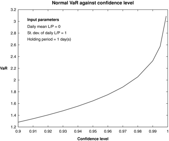
The calculation of VaR and expected tail loss (ETL) with the order statistics methodology can be easily implemented in Matlab. Table 1 contains the VaR and ETL as estimated via the order statistics method for simulated samples using the Gaussian distribution and the t distribution for the series of P/L, at various confidence levels and sample sizes. In addition, the confidence intervals determined as the 0.025% and 0.975% percentiles of the distribution of each risk measure are also included. For a given sample size, the confidence intervals for both VaR and ETL are widening with the increase in the level of confidence, as shown in Figures 1 and 2. Similar results are obtained for larger sample sizes and other distributions. For a prespecified level of confidence, the confidence intervals tend to go narrower with the increase in the sample size.

Figure 1 Expected Tail Loss for Normal P/L versus Level of Confidence When the Sample Size Is 100; Calculations Are Done with Order Statistics

Figure 2 VaR for Normal P/L versus Level of Confidence When the Sample Size Is 100; Calculations Are Done with Order Statistics

JOINT PROBABILITY DISTRIBUTIONS FOR ORDER STATISTICS

If F[i](u) = P(Y[i] ≤ u) is the cumulative distribution function of the i-th order statistic, then it is not difficult to see that F[1](y) = 1−[1−F(y; ϕ)]n and F[n](y) = F[(y; ϕ)]n. Exploiting the fact that we use the quantile as a VaR estimator, Dowd (2001) suggested applying the following known result from order statistics for backtesting purposes

(4)

to derive the cumulative distribution function of this estimator

(5)

In the following we shall denote F(y; ϕ) by F(y), for simplicity. David (1981) pointed to the following useful result giving an analytical formula for the distribution function of the order statistic of order j.

(6)

where is the incomplete beta function and B(a, b) is the beta function. This helps to calculate the pdf function for those distributions that are absolute continuous with respect to a dominant probability measure.1 The probability density function of the j-th order statistics is

(7)

where

DISTRIBUTION-FREE CONFIDENCE INTERVALS FOR VaR

From a practical point of view, without any loss of generality, it is safe to assume that the cumulative distribution function F is strictly increasing. Then, for any α (0, 1) the equation

(8)

has a unique solution. This solution refers to the entire population and it is called the quantile of order α, denoted by zα. The 95% VaR is z0.05.

The order statistics can provide a distribution-free confidence interval for the population quantiles. Thompson (1936) showed that

(9)

This powerful result allows the construction of distribution-free confidence intervals for VaR. For given sample size n and VaR level α, there are many combinations of i and j that make the quantity in (9) larger or equal to 1 − a, the confidence level desired. There may be several combinations of order statistics Y[i], Y[j] that satisfy the relationship (9) and the risk manager may decide to select the combination leading to the shortest confidence interval. Remark that choosing the degree of confidence 1 − a is independent of the level of confidence α for VaR point-estimation. In other words, a 95% confidence interval for the population quantile zα can be calculated for 95% VaR or for 99% VaR.

BIVARIATE ORDER STATISTICS

The risk manager is faced with a dilemma. On one hand the regulators are asking usually for 99%-VaR calculation so that the banks are requested to set aside sufficient capital in order to absorb 99% of all losses. On the other hand, internal models may be used for day-to-day operations to forecast 95% Var. As explained by Brooks and Persand (2002) using an example from Kupiec (1995), the standard error of the 99% VaR can be more than 50% larger than the corresponding standard error for the 95% VaR. This is the case for a model using the Gaussian distribution and it can be even worse for fat tail distributions, with the confidence intervals for the first percentile four times wider than confidence intervals for the fifth percentile. For backtesting purposes it would be ideal to do a joint analysis. Thus, the bivariate joint distribution of two order statistics will provide the confidence regions (two-dimensional sets) for pairs of VaR estimates. For example, the confidence regions for 1% VaR and 5% VaR are recovered from the bivariate joint distribution of where , respectively. This distribution is fully characterized by

(10)

with 1 ≤ i < j ≤ n. The probability on the right side of equation (10) can be interpreted as the probability that at least i values from the entire sample Y1,Y2,…,Yn are not greater than x and at least j values from the same sample Y1,Y2, … ,Yn are not greater than y. Hence

(11)

As in the univariate case, see David (1981), it follows that

(12)

for any x < y. Since for x ≥ y the event {Y[j] ≤ y} implies Y[i] ≤ x then .

An interesting corollary following from this result is that any two order statistics, and therefore VaR estimates at different levels, are not independent. This follows because the joint distribution in (12) cannot be factorized as a product of two factors, one depending only on x and the other only on y, up to a proportionality constant. In other words, if both 1% VaR and 5% VaR, for example, are needed for risk management purposes, then the quality of the VaR estimates should be investigated looking at the joint bivariate distribution like that in (12) rather than separate distributions of the type given in (5).

KEY POINTS

• Order statistics can be used as estimators of VaR and ETL and they are easy to compute.
• Banks may have to work with VaR measures at several levels of confidence because of regulatory requirements that may not coincide exactly with internal risk management decisions.
• ETL can be estimated easily with the framework based on order statistics, as the mean of the sample censored by the VaR threshold.
• For a given sample size, the confidence intervals for both VaR and ETL are widening with the increase in the level of confidence. For a prespecified level of confidence, the confidence intervals tend to go narrower with the increase in the sample size.
• There is a closed form solution for the density of any order statistic, which has been advocated here as a VaR estimator. Therefore, it would be easy to perform backtesting of VaR in this setup.
• The bivariate distribution of any two order statistics is known in closed form and therefore could be used for backtesting when banks have to work with two VaR measures simultaneously.

NOTE

1. For practical cases such as those encountered in finance we can safely assume that the random variables describing P/L series are continuous and they have probability density functions.

REFERENCES

Berkowitz, J., and O’Brien, J. (2002). How accurate are value-at-risk models at commercial banks. Journal of Finance 57, 3: 1093–1111.

Brooks, C., and Persand, G. (2002). Model choice and value-at-risk performance. Financial Analysts Journal 58, 5: 87–97.

David, H. (1981). Order Statistics, 2nd ed. New York: Wiley.

Dowd, K. (2000). Assessing VaR accuracy. Derivatives Quarterly 6, 3: 61–63.

Dowd, K. (2001). Estimating VaR with order statistics. Journal of Derivatives 8, 3: 23–30.

Duffie, D., and Pan, J. (1997). An overview of value-at-risk. Journal of Derivatives 4, 3: 7–49.

Jackson, P., Maude, D. J., and Perraudin, W. (1997). Bank capital and value-at-risk. Journal of Derivatives 4: 73–90.

Jorion, P. (1996). Risk2: Measuring the risk in value-at-risk. Financial Analysts Journal 52: 47–56.

Jorion, P. (1997). Value-at-Risk: The New Benchmark for Controlling Market Risk. Burr Ridge, IL: Irwin.

Kupiec, P. (1995). Techniques for verifying the accuracy of risk measurement models. Journal of Derivatives 3: 73–84.

Marshall, C., and Siegel, M. (1997). Value-at-risk: Implementing a risk measurement standard. Journal of Derivatives 4: 91–110.

Mausser, H. (2001). Calculating quantile-based risk analytics with l-estimators. ALGO Research Quarterly 4, 4: 33–47.

Pritsker, M. (1997). Evaluating VaR methodologies: Accuracy versus computational time. Journal of Financial Services Research 12: 201–241.

Thompson, W. (1936). On confidence ranges for the median and other expectation distributions for populations of unknown distribution form. Annals of Mathematical Statistics 42: 268–269.