Default Correlation in Intensity Models for Credit Risk Modeling

ABEL ELIZALDE, PhD

Credit Derivatives Strategy, J.P. Morgan

There are two primary types of models in the literature that attempt to describe default processes for debt obligations and other defaultable financial instruments, usually referred to as structural and reduced-form (or intensity) models.

Structural models use the evolution of firms’ structural variables, such as asset and debt values, to determine the time of default. Merton’s model (1974) was the first modern model of default and is considered the first structural model. In Merton’s model, a firm defaults if, at the time of servicing the debt, its assets are below its outstanding debt. A second approach within the structural framework was introduced by Black and Cox (1976). In this approach defaults occur as soon as a firm’s asset value falls below a certain threshold. In contrast to the Merton approach, default can occur at any time.

Reduced-form models do not consider the relation between default and firm value in an explicit manner. Intensity models represent the most extended type of reduced-form models.1 In contrast to structural models, the time of default in intensity models is not determined via the value of the firm, but it is the first jump of an exogenously given jump process. The parameters governing the default hazard rate are inferred from market data.

Structural default models provide a link between the credit quality of a firm and the firm’s economic and financial conditions. Thus, defaults are endogenously generated within the model instead of exogenously given as in the reduced approach. Another difference between the two approaches refers to the treatment of recovery rates: Whereas reduced models exogenously specify recovery rates, in structural models the value of the firm’s assets and liabilities at default will determine recovery rates.

This entry focuses on the intensity approach, analyzing various models and reviewing the three main approaches to incorporate credit risk correlation among firms within the framework of reduced-form models.

PRELIMINARIES

In this section, we fix the information and probabilistic framework we need to develop the theory of reduced-form models. After presenting the basic features of reduced models and the motivation of the default intensity through Poisson processes, we apply these concepts to the specification of single firm default probabilities and to the valuation formulas for defaultable and defeault-free bonds. Finally, we analyze the different treatments the recovery rate has received in the literature.

Information Framework

For the purposes of this investigation, we shall always assume that economic uncertainty is modeled with the specification of a filtered probability space , where is the set of possible states of the economic world, and P is a probability measure. The filtration represents the flow of information over time. is a -algebra, a family of events at which we can assign probabilities in a consistent way.2 Before continuing with the exposition, let us make some remarks about the choice of the probability space.

First, we assume, as a starting point, that we can fix a unique physical or real probability measure , and we consider the filtered probability space . The choice of the probability space will vary in some respects, according to the particular problems under consideration. In the rest of the entry, as we indicated above, we shall regularly make use of a probability measure P, that will be assumed to be equivalent to . The choice of P then varies according to the context.

The model for the default-free term structure of interest rates is given by a non-negative, bounded and -adapted default-free short-rate process rt. The money market account value process is given by:

(1)

For our purposes we shall use the class of equivalent probability measures P, where non-dividend-paying (NDP) asset processes discounted by the money market account are -martingales, that is, where P is an equivalent probability measure that uses the money market account as numeraire.3 Such an equivalent measure is called a risk neutral measure, because under this probability measure the investors are indifferent between investing in the money market account or in any other asset. There are different scenarios under which the transition from the physical to the equivalent (or risk neutral) probability measure can usually be accomplished.

We present a mathematical framework that will embody essentially all models used throughout this entry. Nevertheless, more general frameworks can be considered. On our probability space we assume that there exists an -valued Markov process or background process, that represents J economy-wide variables, either state (observable) or latent (not observable).4 There also exist I counting processes, , , initialized at 0, that represent the default processes of the I firms in the economy such that the default of the ith firm occurs when jumps from 0 to 1. and , where and , represent the filtrations generated by Xt and respectively. The filtration represents information about the development of general market variables and all the background information, whereas only contains information about the default status of firm i.

The filtration contains the information generated by both the information contained in the state variables and the default processes:

(2)

We also define the filtrations , , as

(3)

which only accumulate the information generated by the state variables and the default status of each firm.

Poisson and Cox Processes

Poisson processes provide a convenient way of modeling default arrival risk in intensity-based default risk models.5 In contrast to structural models, the time of default in intensity models is not determined via the value of the firm, but instead is taken to be the first jump of a point process (for example, a Poisson process). The parameters governing the default intensity (associated with the probability measure P) are inferred from market data.

First, we recall the formal definition of Poisson and Cox processes. Consider an increasing sequence of stopping times (). We define a counting process associated with that sequence as a stochastic process Nt given by

(4)

A (homogeneous) Poisson process with intensity is a counting process whose increments are independent and satisfy

(5)

for , that is, the increments are independent and have a Poisson distribution with parameter for .

So far, we have considered only the case of homogeneous Poisson processes where the default intensity is a constant parameter , but we can easily generalize it allowing the default intensity to be time dependent , in which case we would talk about unhomogeneous Poisson processes.

If we consider stochastic default intensities, the Poisson process would be called a Cox process. For example, we can assume follows a diffusion process of the form

(6)

where Wt is a Brownian motion. We can also assume that the intensity is a function of a set of state variables (economic variables, interest rates, currencies, etc.) Xt, that is, .

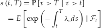
The fundamental idea of the intensity-based framework is to model the default time as the first jump of a Poisson process. Thus, we define the default time to be

(7)

The survival probabilities in this setup are given by

(8)

The intensity, or hazard rate, is the conditional default arrival rate, given no default:

(9)

where

(10)

and is the density of F.

The functions and are the risk neutral default and survival probabilities from time t to time T respectively, where . Note that , and if we fix , then .

The hazard or intensity rate is the central element of reduced form models, and represents the instantaneous default probability, that is, the (very) short-term default risk.

Pricing Building Blocks

This section reviews the pricing of risk-free and defaultable zero-coupon bonds, which together with the default/survival probabilities constitute the building blocks for pricing credit derivatives and defaultable instruments.

We assume a perfect and arbitrage-free capital market, where the money market account value process is given by (1). Since our probability measure P takes as numeraire the money market account process, the value of any NDP-asset discounted by the money market account follows an -martingale. Using the previous property, the price at time t of a default-free zero coupon bond with maturity T and face value of 1 unit is given by

(11)

From the previous section we know that the survival probability in the risk-neutral measure can be expressed as

(12)

Consider a defaultable zero coupon bond issued by firm i with maturity T and face value of M units that, in case of default at time , generates a recovery payment of units. Rt is an -adapted stochastic process, with for all .6 The price of the defaultable coupon bond at time t, , is given by

(13)

which can be expressed as7

(14)

assuming and all the technical conditions that ensure that the expectations are finite.8 This expression has to be evaluated considering the treatment of the recovery payment and any other assumptions about the correlations between interest rates, intensities, and recoveries. The first term represents the expected discounted value of the payment of M units at time T, taking into account the possibility that the firm may default and the M units not received, through the inclusion of the hazard or intensity rate (instantaneous probability of default) in the discount rate. The second term represents the expected discounted value of the recovery payment using the risk-free rate plus the intensity rate as discount factor. The first integral in the second term of the previous expression, from t to T, makes reference to the fact that default can happen at any time between t and T. Thus, for each , we discount the value of the recovery rate Rs times the instantaneous probability of default at time s given that no default has occurred before, which is given by the intensity .

Recovery Rates

Recovery rates refer to how we model, after a firm defaults, the value that a debt instrument has left.9 In terms of the recovery rate parametrization, three main specifications have been adopted in the literature. The first one considers that the recovery rate is an exogenous fraction of the face value of the defaultable bond (recovery of face value, RFV).10 Jarrow and Turnbull (1997) consider the recovery rate to be an exogenous fraction of the value of an equivalent default-free bond (recovery of treasury, RT). Finally, Duffie and Singleton (1999a) fix a recovery rate equal to an exogenous fraction of the market value of the bond just before default (recovery of market value, RMV).

The RMV specification has gained a great deal of attention in the literature thanks to, among others, Duffie and Singleton (1999a). Consider a zero-coupon defaultable bond, which pays M at maturity T if there is no default prior to maturity and whose payoff in case of default is modeled according to the RMV assumption. They show that this bond can be priced as if it were a default-free zero-coupon bond, by replacing the usual short-term interest rate process rt with a default-adjusted short rate process . Lt is the expected loss rate in the market value if default were to occur at time t, conditional on the information available up to time

(15)

(16)

where is the default time, the market price of the bond just before default, and the value of the defaulted bond. Duffie and Singleton (1999a) show that (14) can be expressed as

(17)

This expression shows that discounting at the adjusted rate accounts for both the probability and the timing of default, and for the effect of losses at default. But the main advantage of the previous pricing formula is that, if the mean loss rate does not depend on the value of the defaultable bond, we can apply well-known term structure processes to model instead of rt to price defaultable debt. One of the main drawbacks of this approach is that since appears multiplied in , in order to be able to estimate and Lt separately using data of defaultable instruments, it is not enough to know defaultable bond prices alone. We would need to have available a collection of bonds that share some, but not all, default characteristics, or derivative securities whose payoffs depend, in different ways, on and Lt. In case and Lt are not separable, we shall have to model the product (which represents the short-term credit spread).11 This identification problem is the reason why most of the empirical work that tries to estimate the default intensity process from defaultable bond data uses an exogenously given constant, that is, for all t, recovery rate.12

The previous valuation formula allows one to introduce dependencies between short-term interest rates, default intensities, and recovery rates (via state variables, for example).

From a pricing point of view, the above pricing formula allows us to include the case in which, as is often seen in practice after a default takes place, a firm reorganizes itself and continues with its activity. If we assume that after each possible default the firm is reorganized and the bondholders lose a fraction Lt of the predefault bond’s market value, Giesecke (2002a) shows that letting Lt be a constant, that is, for all t, the price of a default risky zero-coupon bond is, as in the case with no reorganization, given by (17).

Another advantage of this framework is that it allows one to consider liquidity risk by introducing a stochastic process lt as a liquidity spread in the adjusted discount process ; that is, .

SINGLE ENTITY

The aim of this section is to develop some tools in the modeling of intensity processes, in order to build the models for default correlation. In case we consider a deterministic specification for default intensities, it is natural to think of time dependent intensities, in which , where is usually modeled as either a constant, linear, or quadratic polynomial of the time to maturity.13

The treatment of default-free interest rates, the recovery rate, and the intensity process differentiates each intensity model.

It is interesting to note that the difference between the pricing formulas of default-free zero-coupon bonds and survival probabilities in the intensity approach lies in the discount rate:

(18)

(19)

This analogy between intensity-based default risk models and interest rate models allows us to apply well-known short-rate term models to the modeling of default intensities.

Schönbucher (2003) enumerates several characteristics that an ideal specification of the interest rate rt and the default intensity should have. First, both rt and should be stochastic. Second, the dynamics of rt and should be rich enough to include correlation between them. Third, it is desirable to have processes for rt and that remain positive at all times. And finally, the easier the pricing of the pricing building blocks, the better.

We start with a general framework, making use of the Markov process , which represents J state variables. The most general process for Xt that we shall consider is called a basic affine process, which is an example of an affine jump diffusion given by

(20)

for , where is an -Brownian motion. and represent the mean reversion rate and level of the process, and is a constant affecting the volatility of the process. denotes any jump that occurs at time t of a pure-jump process , independent of , whose jump sizes are exponentially distributed with mean and whose jump times are independent Poisson random variables with intensity of arrival (jump times and jump sizes are also independent). By modeling the jump size as an exponential random variable, we restrict the jumps to be positive. This process is called a basic affine process with parameters .14

Making rt and dependent on a set of common stochastic factors Xt, one can introduce randomness and correlation in the processes of rt and . Moreover, if we use basic affine processes for the common factors Xt, we can make use of the following results, which will yield closed-form solutions for the building blocks we examined in the previous section:15

1. For any discount-rate function and any function , if Xt is a Markov process (which holds in the case of basic affine process), then

(21)

for and for some function H : .

2. Defining an affine function as constant plus linear, if and are affine functions ( and ) then, as shown by Duffie, Pan, and Singleton (2000), if Xt is an affine jump-diffusion process, it is verified that can be expressed in closed form by

(22)

for some coefficients which are functions, also in closed form, of the parameters of the model.16

Observing that our pricing building blocks , and are special cases of the previous expressions, one realizes the gains in terms of tractability achieved by the use of affine processes in the modelling of the default term structure.17 In order to make use of this tractability the state variables Xt should follow affine processes, and the specification for the risk-adjusted rate should be an affine function of the state variables.

Consider the case in which the follow (20). If we eliminate the jump component from the process of

(23)

we obtain the CIR process, and eliminating the square root of

(24)

we end up with a Vasicek model.

Various reduced-form models differ from each other in their choices of the state variables and the processes they follow. In the models we consider below, the intensity and interest rate are linear, and therefore affine, functions of Xt, where Xt are basic affine processes.18

One can consider expressions for rt and of the general form

(25)

(26)

for some deterministic (possibly time-dependent) coefficients and , . This type of model allows us to treat rt and as stochastic processes, to introduce correlations between them, and to have analytically tractable expressions for pricing the building blocks. A simple example could be

(27)

(28)

(29)

in which the state variables are rt and themselves, whose Brownian motions are correlated.

Duffie (2005) presents an extensive review of the use of affine processes for credit risk modeling using intensity models, and applies such models to price different credit derivatives (credit default swaps, credit guarantees, spread options, lines of credit, and ratings-based step-up bonds.)

Default Times Simulation

Letting U be a uniform (0,1) random variable independent of , the time of default is defined by

(30)

Equivalently, we can let be an exponentially distributed random variable with parameter 1 and independent of and define the default time as

(31)

Once we have specified and calibrated the dynamics of , we can easily simulate default times using a simple procedure based on the two previous definitions. First, we simulate a realization u of a uniform random variable U and choose such that . Equally, we can simulate a random variable exponentially distributed with parameter 1 and fix such that .

DEFAULT CORRELATION

This section reviews the different approaches to model the default dependence between firms in the reduced-form approach. With the tools provided in the previous section we can calculate the survival or default probability of a given firm in a given time interval. The next natural question to ask ourselves concerns the default or survival probability of more than one firm. If we are currently at time t and no default has occurred so far, what is the probability that different firms default before time T? or, what is the probability that they all survive until time T?

Schönbucher (2003), again, points out some properties that any good approach to model dependent defaults should verify. First, the model must be able to produce default correlations of a realistic magnitude. Second, it has to do it by keeping the number of parameters introduced to describe the dependence structure under control, without growing dramatically with the number of firms. Third, it should be a dynamic model, able to model the number of defaults as well as the timing of defaults. Fourth, since it is clear from the default history that there are periods in which defaults may cluster, the model should be capable of reproducing these periods. And fifth, the easier the calibration and implementation of the model, the better.

We can distinguish three different approaches to model default correlation in the literature of intensity credit risk modeling. The first approach introduces correlation in the firms’ default intensities making them dependent on a set of common variables Xt and on a firm specific factor. These models have received the name of conditionally independent defaults (CID) models, because conditioned to the realization of the state variables Xt, the firm’s default intensities are independent as are the default times that they generate. Apparently, the main drawback of these models is that they do not generate sufficiently high default correlations. However, Yu (2002a) indicates that this is not a problem of the model per se, but rather an indication of the lack of sophistication in the choice of the state variables.

Two direct extensions of the CID approach try to introduce more default correlation in the models. One is the possibility of joint jumps in the default intensities (Duffie and Singleton 1999b) and the other is the possibility of default-event triggers that cause joint defaults (Duffie and Singleton 1999b, Kijima 2000, and Kijima and Muromachi 2000).

The second approach to model default correlation, contagion models, relies on the works by Davis and Lo (1999) and Jarrow and Yu (2001). It is based on the idea of default contagion in which, when a firm defaults, the default intensities of related firms jump upwards. In these models default dependencies arise from direct links between firms. The default of one firm increases the default probabilities of related firms, which might even trigger the default of some of them.

The last approach to model default correlation makes use of copula functions. A copula is a function that links univariate marginal distributions to the joint multivariate distribution with auxiliary correlating variables. To estimate a joint probability distribution of default times, we can start by estimating the marginal probability distributions of individual defaults, and then transform these marginal estimates into the joint distribution using a copula function. Copula functions take as inputs the individual probabilities and transform them into joint probabilities, such that the dependence structure is completely introduced by the copula.

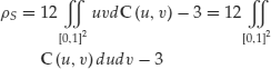
Measures of Default Correlation

The complete specification of the default correlation will be given by the joint distribution of default times. Nevertheless, we can specify some other measures of default correlation. Consider two firms A and B that have not defaulted before time t . We denote the probabilities that firms A and B will default in the time interval by pA and pB respectively. Denote pAB the probability of both firms defaulting before T, and and the default times of each firm. The linear correlation coefficient between the default indicator random variables and is given by

(32)

In the same way we can define the linear correlation of the random variables and . Another measure of default dependence between firms is the linear correlation between the random variables and , .

The conclusions extracted from the comparison of linear default correlations should be viewed with caution because they are covariance-based and hence they are only the natural dependence measures for joint elliptical random variables.19 Default times, default events, and survival events are not elliptical random variables, and hence these measures can lead to severe misinterpretations of the true default correlation structure.20

The previous correlation coefficients, when estimated via a risk neutral intensity model, are based on the risk neutral measure. However, when we calculate the correlation coefficients using empirical default events, the correlation coefficients are obtained under the physical measure. Jarrow, Lando, and Yu (2001) and Yu (2002a, b) provide a procedure for computing physical default correlation through the use of risk neutral intensities.

Conditionally Independent Default Models

From now on, we consider different firms and denote by and their default intensities and default times respectively.

In CID models, firms’ default intensities are independent once we fix the realization of the state variables Xt. The default correlation is introduced through the dependence of each firm’s intensity on the random vector Xt. A firm-specific factor of stochasticity , independent across firms, completes the specification of each firm’s default intensity:

(33)

where are some deterministic coefficients, for and .21

Since default times are continuously distributed, this specification implies that the probability of having two or more simultaneous defaults is zero.

Let us consider an example of a CID model based on Duffee (1999). The default-free interest rate is given by

(34)

where is a constant coefficient, and and are two latent factors (unobservable, interpreted as the slope and level of the default-free yield curve). After having estimated the latent factors and from default-free bond data, Duffee (1999) uses them to model the intensity process of each firm i as

(35)

(36)

where are independent Brownian motions, , , and are constant coefficients, and and are the sample means of and .

The intensity of each firm i depends on the two common latent factors and and on an idiosyncratic factor , independent across firms. The coefficients , , , , and are different for each firm. In Duffee’s model, captures the stochasticity of intensities and the coefficients and , , capture the correlations between intensities themselves, and between intensities and interest rates.

Duffee (1999), Zhang (2003), Driessen (2005), and Elizalde (2005b) propose, and estimate, different CID models.22

The literature on credit risk correlation has criticized the CID approach, arguing that it generates low levels of default correlation when compared with empirical default correlations. However, Yu (2002a) suggests that this apparent low correlation is not a problem of the approach itself but a problem of the choice of state or latent variables, owing to the inability of a limited set of state variables to fully capture the dynamics of changes in default intensities. In order to achieve the level of correlation seen in empirical data, a CID model must include among the state variables the evolution of the stock market, corporate and default-free bond markets, as well as various industry factors.

According to Yu, the problem of low correlation in Duffee’s model may arise because of the insufficient specification of the common factor structure, which may not capture all the sources of common variation in the model, leaving them to the idiosyncratic component, which in turn would not be independent across firms. In fact, Duffee finds that idiosyncratic factors are statistically significant and correlated across firms. As long as the firms’ credit risk depend on common factors different from the interest rate factors, Duffee’s specification is not able to capture all the correlation between firms’ default probabilities. Xie, Wu, and Shi (2004) estimate Duffee’s model for a sample of U.S. corporate bonds and perform a careful analysis of the model pricing errors. A principal component analysis reveals that the first factor explains more than 90% of the variation of pricing errors. Regressing bond pricing errors with respect to several macroeconomic variables, they find that returns on the S&P 500 index explain around 30% of their variations. Therefore, Duffee’s model leaves out some important aggregate factors that affect all bonds.

Driessen (2005) proposes a model in which the firms’ hazard rates are a linear function of two common factors, two factors derived from the term structure of interest rates, a firm idiosyncratic factor, and a liquidity factor. Yu also examines the model of Driessen (2005), finding that the inclusion of two new common factors elevates the default correlation.

Finally, Elizalde (2005b) shows that any firm’s credit risk is, to a very large extent, driven by common risk factors affecting all firms. The study decomposes the credit risk of a sample of corporate bonds (14 U.S. firms, 2001--2003) into different unobservable risk factors. A single common factor accounts for more than 50% of all (but two) of the firms’ credit risk levels, with an average of 68% across firms. Such factor represents the credit risk levels underlying the U.S. economy and is strongly correlated with main U.S. stock indexes. When three common factors are considered (two of them coming from the term structure of interest rates), the model explains an average of 72% of the firms’ credit risk.23

Default Times Simulation

In the CID approach, to simulate default times we proceed as we did in the single entity case. Once we know the realization of the state variables , we simulate a set of I independent unit exponential random variables , which are also independent of . The default time of each firm is defined by

(37)

Thus, once we have simulated , will be such that

(38)

Joint Jumps/ Joint Defaults

Duffie and Singleton (1999b) proposed two ways out of the low correlation problem. One is the possibility of joint jumps in the default intensities, and the other is the possibility of default-event triggers that cause joint defaults.24

Duffie and Singleton develop an approach in which firms experience correlated jumps in their default intensities. Assume that the default intensity of each firm follows the following process:

(39)

which consists of a deterministic mean reversion process plus a pure jump process , whose intensity of arrival is distributed as a Poisson random variable with parameter and whose jump size follows an exponential random variable with mean (equal for all firms ).25 Duffie and Singleton introduce correlation to the firm’s jump processes, keeping unchanged the characteristics of the individual intensities. They postulate that each firm’s jump component consists of two kinds of jumps, joint jumps and idiosyncratic jumps. The joint jump process has a Poisson intensity and an exponentially distributed size with mean . Individual default intensities experience a joint jump with probability pi. That is, a firm suffers a joint jump with Poisson intensity of arrival of . In order to keep the total jump in each firm’s default intensity with intensity of arrival and size , the idiosyncratic jump (independent across firms) is set to have an exponentially distributed size and intensity of arrival hi, such that .

Note that if the jumps are only idiosyncratic jumps, implying that default intensities and hence default times are independent across firms. If and all firms have the same jump intensity, which does not mean that default times are perfectly correlated, since the size of the jump is independent across firms. Only if we additionally assume that goes to infinity we obtain identical default times.

The second alternative considers the possibility of simultaneous defaults triggered by common credit events, at which several obligors can default with positive probability. Imagine there exist common credit events, each one modeled as a Poisson process with intensity . Given the occurrence of a credit event m at time t, each firm i defaults with probability . If, given the occurrence of a common shock, the firm’s default probability is less than one, this common shock is called nonfatal shock, whereas if this probability is one, the common shock is called fatal shock. In addition to the common credit events, each entity can experience default through an idiosyncratic Poisson process with intensity , which is independent across firms. Therefore, the total intensity of firm i is given by

(40)

Consider a simplified version of this setting with two firms, constant idiosyncratic intensities and , and one common and fatal event with constant intensity . In this case firm i’s survival probability is given by

(41)

Denoting by the joint survival probability, given no default until time t, that firm 1 does not default before time T1 and firm 2 does not default before time T2, then

(42)

which can be expressed as

(43)

This expression for the joint survival probability explicitly includes individual survival probabilities and a term that introduces the dependence structure. This is the approach followed by copula functions, which couple marginal probabilities into joint probabilities. In fact, the above example is a special case of copula function, called Marshall-Olkin copula.

The relationship between joint survival and default probabilities is given by

(44)

where represents the joint default probability, given no default until time t, that firm 1 defaults before time T1 and firm 2 defaults before time T2. Obviously the case with multiple common shocks is more troublesome in terms of notation and calibration because, for every possible common credit event, an intensity must be specified and calibrated.26

Duffie and Singleton (1999b) propose algorithms to simulate default times within these two frameworks. The criticisms that the joint credit event approach has received stem from the fact that it is unrealistic that several firms default at exactly the same time, and also from the fact that after a common credit event that makes some obligors default, the intensity of other related obligors that do not default does not change at all.

Although theoretically appealing, the main drawback of these two last models has to do with their calibration and implementation. To the best of my knowledge there is not a single paper that carries out an empirical calibration and implementation of a model like the ones presented in this section. The same applies to the contagion models presented in the next section.

Contagion Mechanisms

Contagion models take CID models one step further, introducing into the model two empirical facts: that the default of one firm can trigger the default of other related firms and that default times tend to concentrate in certain periods of time, in which the default probability of all firms is increased. The last model examined in the previous section (joint credit events) differs from contagion mechanisms in that if an obligor does not experience a default, its intensity does not change due to the default of any related obligor. The literature of default contagion includes two approaches: the infectious defaults model of Davis and Lo (1999), and the model proposed by Jarrow and Yu (2001), which we shall refer to as the propensity model. The main issues to be resolved concerning these two models are associated with difficulties in their calibration to market prices.

The Davis-Lo Infectious Defaults Model

The model developed by Davis and Lo (1999) has two versions, a static version that only considers the number of defaults in a given time period,27 and a dynamic version in which the timing of default is also incorporated. 28

In the dynamic version of the model, each firm has an initial hazard rate of , for , which can be constant, time dependent, or follow a CID model. When a default occurs, the default intensity of all remaining firms is increased by a factor , called the enhancement factor, to . This augmented intensity remains for an exponentially distributed period of time, after which the enhancement factor disappears (). During the period of augmented intensity, the default probabilities of all firms increase, reflecting the risk of default contagion.

The Jarrow-Yu Propensity Model

In order to account for the clustering of default in specific periods, Jarrow and Yu (2001) extend CID models to account for counterparty risk: the risk that the default of a firm may increase the default probability of other firms with which it has commercial or financial relationships. This allows them to introduce extra-default dependence in CID models to account for default clustering. In a first attempt, Jarrow and Yu assume that the default intensity of a firm depends on the status (default/not default) of the rest of the firms (symmetric dependence). However, symmetric dependence introduces a circularity in the model, which they refer to as looping defaults, which makes it extremely difficult and troublesome to construct and derive the joint distribution of default times.

Jarrow and Yu restrict the structure of the model to avoid the problem of looping defaults. They distinguish between primary firms () and secondary firms (). First, they derive the default intensity of primary firms, using a CID model. The primary firm intensities are -adapted and do not depend on the default status of any other firm. If a primary firm defaults, this increases the default intensities of secondary firms, but not the other way around (asymmetric dependence). Thus, secondary firms’ default intensities are given by

(45)

for and , where and are -adapted. represents the part of secondary firm i’s hazard rate independent of the default status of other firms.

Default intensities of primary firms are -adapted, whereas default intensities of secondary firms are adapted with respect to the filtration .

This model introduces a new source of default correlation between secondary firms, and also between primary and secondary firms, but it does not solve the drawbacks of low correlation between primary firms, which CID models apparently imply, because the setting for primary firms is, after all, only a CID model.29

Default Times Simulation

First we simulate the default times for the primary firms exactly as in the case of CID. Then, we simulate a set of I−K independent unit exponential random variables (independent of ), and define the default time of each secondary firm as

(46)

Copulas

In CID and contagion models the specification of the individual intensities includes all the default dependence structure between firms. In contrast, the copula approach separates individual default probabilities from the credit risk dependence structure. The copula function takes as inputs the marginal probabilities and introduces the dependence structure to generate joint probabilities.

Copulas were introduced in 1959 and have been extensively applied to model, among others, survival data in areas such as actuarial science.30

In the rest of this section we review copula theory and its use in the credit risk literature. To make notation simple, assume we are at time and take and (or ) to be the survival and default probabilities, respectively, of firm from time 0 to time . Then

(47)

where denotes the default time of firm i.

A copula function transforms marginal probabilities into joint probabilities. In case we model default times, the joint default probability is given by

(48)

and if we model survival times, the joint survival probability takes the form

(49)

where and are two different copulas.31

The copula function takes as inputs the marginal probabilities without considering how we have derived them. Thus, the intensity approach is not the only framework with which we can use copula functions to model the default dependence structure between firms. Any other approach to model marginal default probabilities, such as the structural approach, can use copula theory to model joint probabilities.

Description

An intuitive definition of a copula function is as follows:32

Copula Function A function is a copula if there are uniform random variables taking values in such that C is their joint distribution function.

A copula function C has uniform marginal distributions, that is,

(50)

for all and .

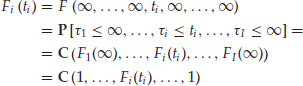
This definition is used, for example, by Schönbucher (2003).33 The copula function C is the joint distribution of a set of I uniform random variables . Copula functions allow one to separate the modeling of the marginal distribution functions from the modeling of the dependence structure. The choice of the copula does not constrain the choice of the marginal distributions. Sklar (1959) showed that any multivariate distribution function F can be written in the form of a copula function. The following theorem is known as Sklar’s theorem:

Sklar’s Theorem Let be random variables with marginal distribution functions and joint distribution function F. Then there exists an I-dimensional copula C such that for all in RI. Moreover, if each Fi is continuous, then the copula C is unique.

We shall consider the default times of each firm as the marginal random variables whose joint distribution function will be determined by a copula function. If Y is a random variable with distribution function F, then the random variable U, defined as , is a uniform random variable. Denoting by ti the realization of each ,34

(51)

The marginal distribution of the default time will be given by

(52)

In the bivariate case, the relationship between the copula and the survival copula , which satisfies , is given by35

(53)

Nelsen (1999) points out that is a copula and that it couples the joint survival function to its univariate margins in a manner completely analogous to the way in which a copula connects the joint distribution function to its margins . When modeling credit risk using the copula framework we can specify a copula for either the default times or the survival times.

Measures of the Dependence Structure

The dependence between the marginal distributions linked by a copula is characterized entirely by the choice of the copula. If and are two I-dimensional copula functions we say that is smaller than , denoted by , if for all .

The Fréchet-Hoeffding copulas, and , are two reference copulas given by36

(54)

(55)

satisfying for any copula C. However, this is a partial ordering in the sense that not every pair of copulas can be compared in this way.

In order to compare any two copulas, we would need an index to measure the dependence structure between two random variables introduced by the choice of the copula function. Linear (Pearson) correlation coefficient is the most used measure of dependence; however, it harbors several drawbacks, which makes it not very suitable to compare copula functions. For example, linear correlation depends not only on the copula but also on the marginal distributions.

We focus on four dependence measures that depend only on the copula function, not in the marginal distributions: Kendall’s tau, Spearman’s rho, and upper/lower tail dependence coefficients.

First, we introduce the concept of concordance:

Concordance Let and be two observations from a vector of continuous random variables. Then, and are said to be concordant if and discordant if .

Kendall’s tau and Spearman’s rho are two measures of concordance:

Kendall’s Tau Let and be IID random vectors of continuous random variables with the same joint distribution function given by the copula C (and with marginals F1 and F2). Then, Kendall’s tau of the vector (and thus of the copula C) is defined as the probability of concordance minus the probability of discordance; that is,

(56)

Spearman’s Rho Let , and be IID random vectors of continuous random variables with the same joint distribution function given by the copula C (and with marginals F1 and ). Then, Spearman’s rho of the vector (and thus of the copula C) is defined as

(57)

Both Kendall’s tau and Spearman’s rho37 take values in the interval and can be defined in terms of the copula function by

(58)

(59)

The Fréchet-Hoeffding copulas take the two extreme values of Kendall’s tau and Spearman’s rho: If the copula of the vector is then , and if it has copula then . The product copula represents independent random variables, that is, if are independent random variables, their copula is given by , such that . For a vector of independent random variables, . Kendall’s tau and Spearman’s rho are equal for a given copula C and its associated survival copula .

Kendall’s tau and Spearman’s rho are measures of global dependence. In contrast, tail dependence coefficients between two random variables are local measures of dependence, as they refer to the level of dependence between extreme values, that is, values at the tails of the distributions and .

Tail Dependence Let be a random vector of continuous random variables with copula C (and with marginals F1 and F2). Then, the coefficient of upper tail dependence of the vector (and thus of the copula C) is defined as

(60)

where represents the inverse function of Fi, provided the limit exists. We say that the random vector (and thus the copula C ) has upper tail dependence if . Similarly, the coefficient of lower tail dependence of the vector (and thus of the copula C) is defined as

(61)

We say that the random vector (and thus the copula C) has lower tail dependence if .

Upper (lower) tail dependence measures the probability that one component of the vector is extremely large (small) given that the other is extremely large (small). As in the case of Kendall’s tau and Spearman’s rho, tail dependence is a copula property and can be expressed as38

(62)

(63)

The upper (lower) coefficient of tail dependence of the copula C is the lower (upper) coefficient of tail dependence of its associated survival copula .

Consider the random vector of default times for two firms. The coefficient of upper (lower) tail dependence represents the probability of long-term survival (immediate joint death). The existence of default clustering periods implies that a copula to model joint default (survival) probabilities should have lower (upper) tail dependence to capture those periods.

Examples of Copulas

Here, we review some of the most used copulas in default risk modeling. The first two copulas, normal and Student t copulas, belong to the elliptical family of copulas. We also present the class of Archimedean copulas and the Marshall-Olkin copula.39

1. Elliptical CopulasThe I-dimensional normal copula with correlation matrix is given by

(64)

where represents an I-dimensional normal distribution function with covariance matrix , and denotes the inverse of the univariate standard normal distribution function.

Normal copulas are radially symmetric (), tail independent (), and their concordance order depends on the linear correlation parameter :

(65)

As with any other copula, the normal copula allows the use of any marginal distribution. We can express the linear correlation coefficients for a normal copula () in terms of both Kendall’s tau () and Spearman’s rho () in the following way:

(66)

Another elliptical copula is the t-copula. Letting X be an random vector distributed as an I-dimensional multivariate t-student with v degrees of freedom, mean vector (for ) and covariance matrix (for ), we can express X as

(67)

where S is a random variable distributed as an with v degrees of freedom and Z is an I-dimensional normal random vector, independent of S, with zero mean and linear correlation matrix . The I -dimensional t-copula of X can be expressed as

(68)

where represents the distribution function of , where Y is an I-dimensional normal random vector, independent of S, with zero mean and covariance matrix R. denotes the inverse of the univariate t-student distribution function with v degrees of freedom and .

The t-copula is radially symmetric and exhibits tail dependence given by

(69)

where is the linear correlation of the bivariate t-distribution.

2. Archimedean CopulasAn I-dimensional Archimedean copula function C is represented by

(70)

where the function , called the generator of the copula, is invertible and satisfies , , . An Archimedean copula is entirely characterized by its generator function. Relevant Archimedean copulas are the Clayton, Frank, Gumbel, and Product copulas, whose generator functions are given by:

Copula	Generator
Clayton		for
Frank		for
Gumbel		for
Product

The Clayton copula has lower tail dependence but not upper tail dependence. The Gumbel copula has upper tail dependence but not lower tail dependence. The Frank copula does not exhibit either upper or lower tail dependence.

Archimedean copulas allow for a great variety of different dependence structures, and the ones presented above are especially interesting because they are one-parameter copulas. In particular, the larger the parameter (in absolute value), the stronger the dependence structure. The Clayton, Frank, and Gumbel copulas are ordered in (i.e., for all ). Unlike the Gumbel copula, which does not allow for negative dependence, Clayton and Frank copulas are able to model continuously the whole range of dependence between the lower Fréchet-Hoeffding copula, the product copula and the upper Fréchet-Hoeffding copula. Copulas with this property are called inclusive or comprehensive copulas. Frank copulas are the only radially symmetric Archimedean copulas ().

For Archimedean copulas, tail dependence and Kendall’s tau coefficients can be expressed in terms of the generator function

(71)

(72)

(73)

provided the derivatives and limits exist.

Archimedean copulas are interchangeable, which means that the dependence between any two (or more) random variables does not depend on which random variables we choose. In terms of credit risk analysis, this imposes an important restriction on the dependence structure since the default dependence introduced by an Archimedean copula is the same between any group of firms.

3. Marshall-Olkin CopulaThis copula was already mentioned when we dealt with joint defaults in intensity models. In its bivariate specification the Marshall-Olkin copula is given by

(74)

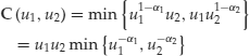
for .40

Copulas for Default Times

Within the reduced-form approach, we can distinguish two approaches to introduce default dependence using copulas. The first one, which we will refer to as Li’s approach, was introduced by Li (1999) and represents one of the first attempts to use copula theory systematically in credit risk modeling. Li’s approach takes as inputs the marginal default (survival) probabilities of each firm and derives the joint probabilities using a copula function.41 Although Li (1999) studies the case of a normal copula, any other copula can be used within this framework.

If we are using a copula function as a joint distribution for default (survival) times, the simulated vector of uniform random variables from the copula will correspond to the default (survival ) marginal distributions. Once we have simulated the vector , we use it to derive the implied default times such that , or in the survival case, for .

The second approach was introduced by Schönbucher and Schubert (2001), and here we shall call it the Schönbucher-Schubert (SS) approach. In the algorithm to draw a default time in the case of a single firm, we simulated a realization ui of a uniform random variable independent of , and defined the time of default of firm i as such that

(75)

where is the default intensity process of firm i. The idea of the SS approach is to link the default thresholds with a copula.

Schönbucher and Schubert consider that the processes are -adapted42 and call them pseudo default intensities. Thus, is the default intensity if investors only consider the information generated by the background filtration and by the default status of firm i, . However, investors are not restricted to the information represented by as they also observe the default status of the rest of the firms. Therefore, is not the density of default with respect to all the information investors have available, as represented by , but rather with respect to a smaller information set.

To calculate the default (or survival) probabilities conditional to all the information that investors have available, , we cannot define those probabilities in terms of the pseudo default intensities . We have to find the “real” intensities implied by the investors’ information set. The difference between pseudo and real intensities lies in the fact that real intensities, in addition to all the information considered by pseudo intensities, include information about the default status of all firms. The default thresholds’ copula function includes this information in the SS approach.

In order to find the “real” default intensities , which are -adapted, we need to combine both the pseudo default intensities and the copula function, which links the default thresholds. The pseudo default intensity includes information about the state variables and the default situation of firm i, and only coincides with the “real” default intensity hi in cases of independent default or when the information of the market is restricted to .43

The simulation of the default times in this approach is exactly the same as in Li’s approach. The only difference with the SS approach is that it allows us to recover the dynamics of the “real” default intensities , which include the default contagion effects implicit in the default threshold copula. In contrast to the models of Jarrow and Yu (2001) and Davis and Lo (1999), the SS approach allows the contagion effects to arise endogenously through the use of the copula.

Schönbucher (2003) calls the SS approach a dynamic approach in the sense that it considers the dynamics of the “real” default intensities , as opposed to Li’s approach, which only considers the dynamics of the pseudo default intensities.

As Schönbucher and Schubert (2001) point out, this setup is very general, and the reader has freedom to choose the specification of the default intensities. We can introduce default correlation by both correlating the default intensities, for example with a CID model, and by using any of the copula approaches we have just presented.

In an extension of the SS approach, Rogge and Schönbucher (2003) propose not to use the normal or t-copulas but Archimedean copulas, arguing that normal and t-copulas do not imply a realistic dynamic process for default intensities.

Galiani (2003) provides a detailed analysis of the use of copula functions to price multiname credit derivatives using both a normal and Student t copula.

Choosing and Calibrating the Copula

Once we have reviewed how to use copula theory in the context of joint default probabilities, we have to choose a copula and estimate its parameters. In order to choose a copula we should consider aspects such as the dependence structure each copula involves as well as the number of parameters we need to estimate.

Since the normal copula presents neither lower nor upper tail dependence, the use of multivariate normal distributions to model default (or price) behavior has been strongly criticized for not assigning enough probability to the occurrence of extreme events and, among them, the periods of default clustering. The use of the t-copula is the natural answer to the lack of tail dependence, since, subject to the degrees of freedom and covariance matrix, this copula exhibits tail dependence. The main problem in using a normal or t-copula is the number of parameters we have to estimate, which grows with the dimensionality of the copula.44

Archimedean copulas are especially attractive because there exists a large number of one-parameter Archimedean copulas45 which allows for a great variety of dependence structures. The disadvantage of Archimedean copulas is that they may impose too much dependence structure in the sense that, as they are interchangeable copulas, the dependence between any group of firms is the same independently of the firms we consider.

In case we decide to use an Archimedean copula, Genest and Rivest (1993) propose a procedure for identifying the Archimedean copula that best fits the data.46 The problem is that they consider only the bivariate case and that, as we shall see later, we need a sample of the marginal random variables (the random variables whose marginal distributions we link to the copula function) that is available if we are modeling equity returns, but not if we are modeling default times. More generally, Fermanian and Scaillet (2004) discuss the issue of choosing the copula that best fits a given data set, using goodness-of-fit tests.

According to Durrleman, Nikeghbali, and Roncalli (2000):

There does not exist a systematic rigorous method for the choice of the copula: nothing can tell us that the selected family of copula will converge to the real structure dependence underlying the data. This can provide biased results since according to the dependence structure selected the obtained results might be different.

Jouanin et al. (2001) use the term model risk to denote this uncertainty in the choice of the copula.

Assuming we manage to select a copula function, we now face the estimation of its parameters. The main problem of the use of copula theory to model credit risk is the scarcity of default data from which to calibrate the copula.

We cannot rely on multiname credit derivatives, such as ith-to-default products, to calibrate the copula because, in most cases, they are not publicly traded and also because of their lack of liquidity.

Imagine that, instead of fitting a copula to default times, we are fitting a copula to daily stock returns for I different firms. Let be random variables denoting the daily returns of firms with marginal distribution functions and joint distribution function F. Sklar’s theorem proves that there exists an I-dimensional copula C such that for all in RI. In this case, we have available, for each day, a sample of the random vector that we can use to estimate the parameters of the copula. We would have to estimate the parameters of the marginal distribution functions and then estimate the parameters of the copula. Since, in our application to default times, we already have the marginal distributions, determined by the specification of the marginal default intensities, we are left with the estimation of the copula parameters. Providing we have a large sample of the random variables , we can estimate the copula parameters in several ways.47

If the copula is differentiable we can always use maximum likelihood to estimate the parameters.48 De Matteis (2001) mentions that this parametric method may be convenient when we work with a large data set, but in case there are outliers or if the marginal distributions are heavy tailed, a nonparametric approach may be more suitable.

A nonparametric approach would involve the use of the sample version of a dependence measure, such as Kendall’s tau or Spearman’s rho (or both), 49 to calibrate the copula parameters. However, this nonparametric approach is restricted to the bivariate case, and we would need to have at least the same sample dependence measures as copula parameters.50

The estimation methods exposed above rely on the availability of a large sample of the random variables . However, this is not the case when we work with default times. We do not have available a large sample of default times for the I firms. In fact, we do not have a single realization of the default times random vector.

One solution is to assume that the marginal default (survival) probabilities and the marginal distributions of the equity returns share the same copula, that is, share the same dependence structure, and use equity returns to estimate the copula parameters. But this shortcut has its own drawbacks. We need to fit a copula to a set of given marginal distributions for the default (survival) times, which are characterized by a default intensity for each firm. Ideally we should estimate the parameters of the copula function using default times data. However, we rarely have enough default times data available such as to properly estimate the parameters of the copula function. In those cases, we must rely on other data sources to calibrate the copula function. For example, a usual practice is to calibrate the copula using equity data of the different firms. However, the dependence of the firms’ default probabilities will probably differ from the dependence in the evolution of their equity prices.

Another way of dealing with the estimation of the copula parameters is, as Jouanin et al. (2001) propose, through the use of “original methods that are based on the practice of the credit market rather than mimicking statistical methods that are never used by practitioners.” They suggest a method based on Moody’s diversity score.51 The diversity score or binomial expansion technique consists of transforming a portfolio of (credit dependent) defaultable bonds on an equivalent portfolio of uncorrelated and homogeneous credits assumed to mimic the default behavior of the original portfolio, using the so-called diversity score parameter, which depends on the degree of diversification of the original portfolio. We then match the first two moments of the number of defaults within a fixed time horizon for both the original and the transformed portfolio. Since the original portfolio assumes default dependence, the distribution of the number of defaults will depend on the copula parameters. In the transformed portfolio, that is, independent defaults, the number of defaults follows a binomial distribution with some probability p. Matching the first two moments of the number of defaults in both portfolios, we would extract an estimation for the probability p and for the copula parameters.52 However, Moody’s diversity score approach has its own drawbacks. Among others, it is a static model with a fixed time horizon, that is, it does not consider when defaults take place but only the number of defaults within the fixed time horizon. In fact, the Committee on the Global Financial System (Bank for International Settlements) suggests, in its last report,53 that diversity scores “are a fairly crude measure of the degree of diversification in a portfolio of credits.”

Similarly to the choice of the copula function, there does not exist a rigorous method to estimate the parameters of the copula. We can talk about parameter risk which, together with the model risk mentioned earlier, are the principal problems we face if we use the copula approach in the modeling of dependent defaults.

KEY POINTS

• There are two primary types of models in the literature that attempt to describe default processes: structural and reduced-form models. Intensity models represent the most extended type of reduced-form models. In contrast to structural models, the time of default in intensity models is not determined via the value of the firm, but it is the first jump of an exogenously given jump process. The fundamental idea of the intensity-based framework is to model the default time as the first jump of a Poisson process. The default intensity of the Poisson process, also referred to as the hazard rate, can be deterministic (constant or time dependent) or stochastic.
• We review three different ways of introducing default correlations among firms in the framework of intensity models: the conditionally independent defaults (CID) approach, contagion models, and copula functions.
• CID models generate credit risk dependence among firms through the dependence of the firms’ intensity processes on a common set of state variables. Firms’ default rates are independent once we fix the realization of the state variables. Different CID models differ in their choices of the state variables and the processes they follow. Extensions of CID models introduce joint jumps in the firms’ default processes or common default events.
• Contagion models extend the CID approach to account for the empirical observation of default clustering (periods in which firms’ credit risk increases simultaneously and in which the majority of defaults take place). They are based on the idea that, when a firm defaults, the default intensities of related firms jump (upwards), that is, the default of one firm increases the default probabilities of other firms (to the point of potentially causing the default of some of them). These models include, on the specification of default intensities, the existence of contagion sources among firms, which can be explained by either their commercial/financial relationships or simply by their common exposure to the economy.
• In CID and contagion models the specification of the individual intensities includes all the default dependence structure between firms. In contrast, the copula approach separates individual default probabilities from the credit risk dependence structure.
• A copula is a function that links univariate marginal distributions to the joint multivariate distribution function. The copula approach takes as given the marginal default probabilities of the different firms and plugs them into a copula function, which provides the model with the dependence structure to generate joint default probabilities. This approach separates the modeling and estimation of the individual default probabilities, determined by the default intensity processes, from the modeling and calibration or estimation of the device that introduces the credit risk dependence, the copula.

NOTES

1. Brody, Hughston, and Macrina (2007) present an alternative reduced-form model based on the amount and precision of the information received by market participants about the firm’s credit risk. Such a model does not require the use of default intensities; it belongs to the reduced-form approach because (like intensity models) it relies on market prices of defaultable instruments as the only source of information about the firms’ credit risk.

2. An event is a subset of , namely a collection of possible outcomes. -algebras are models for information, and filtrations models for flows of information.

3. For some applications we may wish to enlarge this category of probability measures by relaxing the martingale condition to a local martingale condition, though this point does not concern us in what follows.

4. Given the filtered probability space , an -adapted process Xt is a Markov process with respect to if

with probability one, for all , and for every bounded function f. This means that the conditional distribution at time s of , given all available information, depends only on the current state .

5. For a more detailed exposition see Lando (1994) and Chapter 5 in Schönbucher (2003).

6. This specification of the recovery rate incorporates all possible ways of dealing with recovery payments considered in the literature. Here we consider a continuous version of the recovery rate, that is, Rt is measured and received precisely at the default time. In the discrete version of the recovery rate, Rt is measured and received on the first date after default among a prespecified list of times, where Tn is the maturity date T.

7. See Hughston and Turnbull (2001).

8. See proof on Lando (1994, Proposition 3.1) and Bielecki and Rutkowski (2002, Proposition 8.2).

9. For an extensive review of the treatment of recovery rates see Chapter 6 in Schönbucher (2003).

10. Houweling and Vorst (2001) consider the RFV specification for pricing credit default swaps.

11. See Duffie and Singleton (1999a) and Jarrow (1999).

12. There exist some empirical works that, under some specifications of and rt, find that the value of the recovery rate does not substantially affect the results, as long as the recovery rate lies within a logical interval. See, for instance, Houweling and Vorst (2001) and Elizalde (2005a).

13. See Houweling and Vorst (2001) and Elizalde (2005a) for a comparison of different specifications of (deterministic) time-dependent intensity rates.

14. For a detailed description of affine processes see Duffie and Kan (1996), Duffie (1998), Duffie, Pan, and Singleton (2000), Duffie, Filipovic, and Schachermayer (2002), and Appendix A in Duffie and Singleton (2003). An affine jump-diffusion process is a jump-diffusion process for which the drift vector, instantaneous covariance matrix, and jump intensities all have affine dependence on the state vector. If Xt is a Markov process in some space state , Xt is an affine jump-diffusion if it can be expressed as

where Wt is an -Brownian motion in , , and q is a pure jump process whose jumps have a fixed probability distribution on and arrive with intensity , for some constant . That is, the drift vector , instantaneous covariance matrix and jump intensities all have affine dependence on the state vector Xt. Intuitively this means that, conditional on the path of Xt, the jump times of q are the jump times of a Poisson process with time varying-intensity , and that the size of the jump at time T is independent of and has the probability distribution .

15. See Duffie and Kan (1996) and Duffie, Pan, and Singleton (2000).

16. For the basic affine model, the coefficients can be calculated explicitly. See Duffie and Garleanu (2001), Appendix A in Duffie and Singleton (2003), and Duffie, Pan, and Singleton (2000) for details and extensions.

17. Duffie, Pan, and Singleton (2000) developed a similar closed-form expression to the second term of the price of a defaultable zero-coupon bond

Using their expression, the pricing of defaultable zero-coupon bonds with constant recovery of face value reduces to the computation of a one-dimensional integral of a known function.

18. Several versions of the modeling of rt and in this framework can be found in Duffie, Schroder, and Skidas (1996), Duffee (1999), Duffie and Singleton (1999, 2003), Kijima (2000), Kijima and Muromachi (2000), Duffie and Garleanu (2001), Bielecki and Rutkowski (2002), and Schönbucher (2003). For the estimation of an affine process intensity model without jumps see Duffee (1998) and Duffie, Pedersen, and Singleton (2003).

19. If Y is an n-dimensional random vector and, for some and some n x n nonnegative definite, symmetric matrix , the characteristic function of is a function of the quadratic form , . We say that Y has an elliptical distribution with parameters , and . For example, normal and Student t distributions are elliptical distributions. For a more detailed treatment of elliptical distributions see Bingham and Kiesel (2002) and references cited therein.

20. See Embrechts, McNeal, and Straumann (1999) and Embrechts, Lindskog, and McNeil (2001).

21. We can always consider a model such as

for each firm and introduce correlation via the Browian motions .

22. Duffee (1999), Driessen (2005), and Elizalde (2005b) use latent variables instead of state variables. Collin-Dufresne, Goldstein, and Martin (2001) show that financial and economic variables cannot explain the correlation structure of intensity processes. Latent factors are modeled as affine diffusions and estimated through a maximum likelihood procedure based on the Kalman filter.

23. While Driessen (2005) considers that all firms with the same rating are affected in the same way by common factors, Elizalde (2005b) allows for the effect of each common factor to differ across firms, which increases the flexibility of the credit risk correlation structure.

24. See also Kijima (2000), Kijima and Muromachi (2000), and Giesecke (2002b).

25. This is a basic affine process with parameters .

26. See Embrechts, Lindskog, and McNeil (2001) and Giesecke (2002b).

27. Extending the diversity score (or binomial expansion technique) of Moody’s.

28. This dynamic version is introduced in Davis and Lo (2001).

29. See Yu (2002a) and Frey and Backhaus (2003) for an extension of the Jarrow and Yu (2001) model.

30. See Sklar (1959) and Frees and Valdez (1998).

31. Note that and .

32. For a more detailed description of copula theory see Joe (1997), Frees and Valdez (1998), Nelsen (1999), Costinot, Roncalli, and Teiletche (2000), Embrechts, Lindskog, and McNeil (2001), De Matteis (2001), and Georges et al. (2001).

33. A more formal definition would be the following (Frey, McNeil, and Nyfeler 2001): An I-dimensional copula C is a function with the following properties:

• Grounded: For all , if at least one coordinate , .
• Reflective: If all coordinates of u are 1 except uj then , .
• I-increasing: The C-volume of all hypercubes with vertices in is positive, i.e.

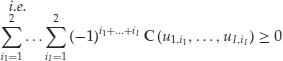
for all and in with for all .

34. We will use , or simply C, to denote the copula function of default times and for the copula function of survival times.

35. See Georges et al. (2001) for a complete characterization of the relation between default and survival copulas.

36. is always a copula, but is only a copula for .

37. A simple interpretation of Spearman’s rho is the following. Let be a random vector of continuous random variables with the same joint distribution function H (whose margins are F1 and ) and copula C, and consider the random variables and . Then, we can write the Spearman’s rho coefficient of as

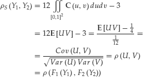
where denotes the Pearson or linear correlation coefficient. So the Spearman’s rho of the vector is the Pearson correlation of the random variables and .

38. Since can be written as

we can express as

39. See Embrechts, Lindskog, and McNeil (2001) and Nelsen (1999) for a more detailed description.

40. For a multivariate version of the Marshall-Olkin copula, see Embrechts, Lindskog, and McNeil (2001).

41. Li (1999) considers a copula that links individual survival probabilities to model the joint survival probability. However, as we have explained previously, this can be done exactly in the same way if we consider default probabilities instead of survival probabilities.

42. Remember that is the information generated by the state variables plus the information generated by the default status of firm i.

43. This distinction between pseudo and real default intensities can also be found in Gregory and Laurent (2002).

44. If we are considering I firms, the number of parameters of the normal copula will be , and we have to add the degrees of freedom parameter in the case of the t-copula.

45. See Nelsen (1999).

46. See also De Matteis (2001) and Frees and Valdez (1998).

47. For a more detailed description of copula parameters estimation see Frees and Valdez (1998), Bouyé et al. (2000), Durrleman, Nikeghbali, and Roncalli (2000), De Matteis (2001), and Patton (2002).

48. We have to distinguish the case in which we estimate the parameters of the marginal distributions and the copula function altogether from the case in which we first estimate the parameters of the marginal distributions and then, using those parameters, we estimate the parameters of the copula function. The latter approach is called inference functions for margins or the IFM method.

49. Imagine we have N random samples of a bivariate vector , let us denote them by , . The sample estimators of Kendall’s tau () and Spearman’s rho () are given by:

where c and are the number of concordant and discordant pairs, respectively.

50. In some cases analytical expressions for the dependence measures are available. Otherwise we have to use a root-finding procedure.

51. For a detailed description of the diversity score method see Cifuentes, Murphy, and O’Connor (1996), Cifuentes and O’Connor (1996), and Cifuentes and Wilcox (1998).

52. See Jouanin et al. (2001).

53. See Committee on the Global Financial System (2003).

REFERENCES

Bielecki, T. R., and Rutkowski, M. (2002). Credit Risk: Modeling, Valuation and Hedging. Springer Finance.

Bingham, N. H., and Kiesel, R. (2002). Semi-parametric modelling in finance: Theoretical foundations. Quantitative Finance 2, 241--250.

Black, F., and Cox, J. C. (1976). Valuing corporate securities: Some effects of bond indenture provisions. Journal of Finance 31, 351--367.

Bouyé, E., Durrleman, V., Nikeghbali, A., Riboulet, G., and Roncalli, T. (2000). Copulas for finance: A reading guide and some applications. Working Paper, Groupe de Recherche Opérationnelle, Crédit Lyonnais, France.

Brody, D., Hughston, L., and Macrina, A. (2007). Beyond hazard rates: A new framework for credit-risk modelling, Advances in Mathematical Finance Edited by Fu, M. C., Jarrow, R. A., Yen, J., and Elliott, R. J. pp: 231–257.

Cifuentes, A., Murphy, E., and O’Connor, G. (1996). Emerging market collateralized bond obligations: An overview. Special Report, Moody’s Investor Service.

Cifuentes, A., and O’Connor, G. (1996). The binomial expansion method applied to CBO/CLO analysis. Special Report, Moody’s Investor Service.

Cifuentes, A., and Wilcox, C. (1998). The double binomial method and its application to a special case of CBO structures. Special Report, Moody’s Investor Service.

Collin-Dufresne, P., Goldstein, R. S., and Martin, J. S. (2001). The determinants of credit spread changes. Journal of Finance 56, 2177--2207.

Committee on the Global Financial System (2003). Credit risk transfer. Bank for International Settlements.

Costinot, A., Roncalli, T., and Teiletche, J. (2000). Revisiting the dependence between financial markets with copulas. Working Paper, Groupe de Recherche Opérationnelle, Crédit Lyonnais, France.

Davis, M., and Lo, V. (1999). Modelling default correlation in bond portfolios. Working Paper, Tokyo-Mitsubitshi International.

Davis, M., and Lo, V. (2001). Infectious defaults. Quantitative Finance 1, 382--386.

De Matteis, R. (2001). Fitting copulas to data. Diploma Thesis, Institute of Mathematics of the University of Zurich.

Driessen, J. (2005). Is default event risk priced in corporate bonds? Review of Financial Studies 18, 165--195.

Duffee, G. R. (1998). The relation between Treasury yields and corporate bond yield spreads. Journal of Finance 53, 65--79.

Duffee, G. R. (1999). Estimating the price of default risk. Review of Financial Studies 12, 197--226.

Duffie, D. (2005). Credit risk modelling with affine processes. Journal of Banking and Finance 29, 2751–2802.

Duffie, D., Filipovic, D., and Schachermayer, W. (2003). Affine processes and applications in finance. Annals of Applied Probability 13, 984–1053.

Duffie, D., and Garleanu, N. (2001). Risk and valuation of collateralized debt obligations. Working Paper, Graduate School of Business, Stanford University.

Duffie, D., and Kan, R. (1996). A yield factor model of interest rates. Mathematical Finance 6, 379--406.

Duffie, D., Pan, J., and Singleton, K. J. (2000). Transform analysis and asset pricing for affine jump diffusions. Econometrica 68, 1343--1376.

Duffie, D., Pedersen, L. H., and Singleton, K. J. (2003). Modeling sovereign yield spreads: A case study of Russian debt. Journal of Finance 58, 119--160.

Duffie, D., Schroder, M., and Skidas, C. (1996). Recursive valuation of defaultable securities and the timing of resolution of uncertainty. Annals of Applied Probability 6, 1075--1090.

Duffie, D., and Singleton, K. J. (1999a). Modeling term structures of defaultable bonds. Working Paper, Graduate School of Business, Stanford University.

Duffie, D., and Singleton, K. J. (1999b). Simulating correlated defaults. Working Paper, Graduate School of Business, Stanford University.

Duffie, D., and Singleton, K. J. (2003). Credit risk: Pricing, measurement and management. Princeton Series in Finance.

Durrleman, V., Nikeghbali, A., and Roncalli, T. (2000). Which copula is the right one? Working Paper, Groupe de Recherche Opérationnelle, Crédit Lyonnais, France.

Embrechts, P., Lindskog, F., and McNeil, A. (2001). Modelling dependence with copulas and applications to risk management. Working Paper, Department of Mathematics, ETHZ, Zurich.

Embrechts, P., McNeal, A., and Straumann, D. (1999). Correlation and dependence in risk management: Properties and pitfalls. Working Paper, Risklab, ETHZ, Zurich.

Elizalde, A. (2005a). Credit default swap valuation: An application to Spanish firms. Available at www.abelelizalde.com.

Elizalde, A. (2005b). Do we need to worry about credit risk correlation? Journal of Fixed Income 15: 3, 42--59.

Fermanian, J., and Scaillet, O. (2004). Some statistical pitfalls in copula modelling for financial applications. FAME Research Paper No. 108.

Frees, E. W., and Valdez, E. A. (1998). Understanding relationships using copulas. North American Actuarial Journal 2, 1--25.

Frey, R., and Backhaus, J. (2003). Interacting defaults and counterparty risk: A Markovian approach. Working Paper, Department of Mathematics, University of Leipzig.

Frey, R., McNeil, A. J., and Nyfeler, M. A. (2001). Copulas and credit models. Working Paper, Department of Mathematics, ETHZ, Zurich.

Galiani, S. (2003). Copula functions and their application in pricing and risk managing multivariate credit derivative products. Master Thesis, King’s College London.

Genest, C., and Rivest, L. P. (1993). Statistical inference procedures for bivariate archimedean copulas. Journal of the American Statistical Association 88, 1034--1043.

Georges, P., Lamy, A. G., Nicolas, E., Quibel, G., and Roncalli, T. (2001). Multivariate survival modelling: A unified approach with copulas. Working Paper, Groupe de Recherche Opérationnelle, Crédit Lyonnais, France.

Giesecke, K. (2002a). Credit risk modelling and valuation: An introduction. Working Paper, Humboldt-Universität, Berlin.

Giesecke, K. (2002b). An exponential model for dependent defaults. Working Paper, Humboldt-Universität, Berlin.

Gregory, J., and Laurent, J. P. (2002). Basket default swaps, CDO’s and factor copulas. Working Paper, BNP Paribas.

Houweling, P., and Vorst, A. C. F. (2001). An empirical comparison of default swap pricing models. Working Paper, Erasmus University Rotterdam.

Hughston, L. P., and Turnbull, S. (2001). Credit risk: Constructing the basic building blocks. Economic Notes 30, 281--292.

Hull, J., and White, A. (2001). Valuing credit default swaps II: Modelling default correlations. Journal of Derivatives 8, 12--22.

Jarrow, R. (1999). Estimating recovery rates and pseudo default probabilities implicit in debt and equity prices. Financial Analysts Journal 57, 75--92.

Jarrow, R., Lando, D., and Turnbull, S. (1997). A Markov model for the term structure of credit risk spreads. Review of Financial Studies 10, 481--523.

Jarrow, R., Lando, D., and Yu, F. (2001). Default risk and diversification: Theory and applications. Working Paper, University of California, Irvine.

Jarrow, R., and Turnbull, S. (1995). Pricing derivatives on financial securities subject to credit risk. Journal of Finance 50, 53--86.

Jarrow, R., and Yu, F. (2001). Counterparty risk and the pricing of defaultable securities. Journal of Finance 56, 1765--1799.

Jamshidian, F. (2002). Valuation of credit default swaps and swaptions. Working Paper, NIB Capital Bank.

Joe, H. (1997). Multivariate models and dependence concepts. Monographs on Statistics and Applied Probability 73, Chapman and Hall, London.

Jouanin, J. F., Rapuch, G., Riboulet, G., and Roncalli, T. (2001). Modelling dependence for credit derivatives with copulas. Working Paper, Groupe de Recherche Opérationnelle, Crédit Lyonnais, France.

Kijima, M. (2000). Valuation of a credit swap of the basket type. Review of Derivatives Research 4, 81--97.

Kijima, M., and Muromachi Y. (2000). Credit events and the valuation of credit derivatives of basket type. Review of Derivatives Research 4, 55--79.

Lando, D. (1994). On Cox processes and credit risky securities. Chapter 3, Ph.D. Thesis, Cornell University.

Li, D. X. (1999). On default correlation: A copula function approach. Working Paper 99--07, The Risk Metrics Group.

Longstaff, F., and Schwartz, E. (1995). A simple approach to valuing risky and floating rate debt. Journal of Finance 50, 781--819.

Madam, D., and Unal, H. (1998). Pricing the risks of default. Review of Derivatives Research 2, 121--160.

Marshall, A., and Olkin, I. (1988). Families of multivariate distributions. Journal of the American Statistical Association 83, 834--841.

Merton, R. (1974). On the pricing of corporate debt: The risk structure of interest rates. Journal of Finance 29, 449--470.

Nelsen, R. B. (1999). An introduction to copulas. Lecture Notes in Statistics 139, Springer-Verlag, New York.

Patton, A. J. (2002). Estimation of copula models for time series of possibly different lengths. Working Paper, University of California, San Diego.

Rogge, E., and Schönbucher, P. J. (2003). Modelling dynamic portfolio credit risk. Working Paper, Department of Statistics, Bonn University.

Schönbucher, P. J. (2003). Credit derivatives pricing models. Wiley Finance.

Schönbucher, P. J., and Schubert, D. (2001). Copula-dependent default risk in intensity models. Working Paper, Department of Statistics, Bonn University.

Sklar, A. (1959). Fonctions de repartition a n dimensions et leurs marges. Publ. Inst. Stat. Univ. Paris 8, 229--231.

Xie, Y., Wu, C., and Shi, J. (2004). Do macroeconomic variables matter for the pricing of default risk? Evidence from the residual analysis of the reduced-form model pricing errors. Presented at 2004 FMA Annual Meeting Program.

Yu, F. (2002a). Correlated default in reduced-form models. Working Paper, University of California, Irvine.

Yu, F. (2002b). Modelling expected return on defaultable bonds. Journal of Fixed Income 12, 69--81.

Zhang, F. X. (2003). What did the credit market expect of Argentina default? Evidence from default swap data. Working Paper, Federal Reserve Board, Division of Research and Statistics, Washington.