
Introduction to Stochastic Programming and Its Applications to Finance
The dynamic nature of financial decision making requires the use of tools that are capable of capturing the multiperiod nature inherent in problems faced by asset managers in portfolio selection decisions and financial managers in capital budgeting decisions. These tools should be understandable with adequate treatment of uncertainty. They should incorporate practical considerations, such as transaction costs in the case of asset managers. Stochastic programming bears these characteristics. In this entry, we discuss the basics of stochastic programming, give a brief history, and emphasize its importance by comparing the approach to other tools used in finance.
WHAT IS STOCHASTIC PROGRAMMING?
Stochastic programming is nothing but a fancy name for the study of optimal decision making under uncertainty. As opposed to “deterministic,” the term “stochastic” implies that some of the parameters of the problem are random (that is, not known with certainty); the term “programming” points to links with mathematical programming and optimization algorithms.
Uncertainty is almost always inherent in real-world decision problems (and even more so in financial planning). As an example, we may consider a bet whose outcome is determined by flipping a coin. In such problems, uncertainty of parameters may be due to the presence of uncertain events (e.g., a coin flip in the previous example) or simply due to lack of reliable data.
In the past, due to computational and informational limitations, optimal decision models were often formulated deterministically by replacing the uncertainties with expectations or best estimates. With contributions from many disciplines, including operations research, and improvements in the information technology (faster hardware and software), stochastic programming is rapidly developing today.
The main features of a stochastic program, which can be viewed as an optimal decision model with explicit consideration of uncertainties, are:
- Random parameters with known (or partially known) distributions.
- Several decision variables with many potential values.
- Discrete time periods for decisions.
- Use of expectations (or other functions of decision variables) for objectives.
The problem structure, constraints, and objectives (risk/reward) are modeled across time along with the uncertainty of events. Future uncertainty is modeled through generating scenarios over time. In other words, the realizations of the uncertain parameters may be (gradually) revealed after some or all of the decisions have been made. High-performance computers take advantage of sophisticated algorithms to determine the optimal decision that will take into account the future uncertainty. As the uncertainty is revealed after each stage, recourse decisions can be made in the light of new information.
The relative importance of these main features contrasts with other decision-making models, such as statistical decision theory, decision analysis, dynamic programming, Markov decision processes, and stochastic control (SC). In contrast to statistical decision theory, stochastic programming has emphasized solution methods and analytical solution properties over procedures for constructing objectives and updating probabilities. Stochastic programs generally have higher dimensions (that is, larger problem size) than SC models, which put more emphasis on control rules and have more restrictive constraint assumptions.
We can see the first forms of decision models that involve uncertainty in the early days of the history of mathematical programming. Beale (1955), Dantzig (1955), and Charnes and Cooper (1959) were the first to propose linear programs with random parameters. Dantzig named his approach “linear programming under uncertainty,” whereas Charnes and Cooper called theirs “chance/probabilistically constrained programming.”
Subsequently, stochastic programming has become a major subfield of mathematical programming with several theoretical developments. For overviews of the literature including algorithms and applications, see Kall and Wallace (1994), Infanger (1994), Ermoliev and Wets (1988), Birge and Louveaux (1997), Wallace and Ziemba (2003), Prékopa (1995), Higle and Sen (1996), Wallace et al. (1996), Censor and Zenios (1997), Wets and Ziemba (1999), Dupačová et al. (2002), Birge et al. (2002), and Ruszczy![]() ski and Shapiro (2003).
ski and Shapiro (2003).
In general, stochastic optimization models result in large-scale programs since they include a large number of scenarios to reflect all possible outcomes of future uncertainty. Therefore, efforts on the algorithmic developments focused on adaptations of large-scale linear programming methods for special classes of stochastic programs whose structures are exploitable. In other words, emphasis was placed on forming the deterministic equivalent program and taking advantage of the structure of the resulting formulation. Dantzig and Madansky (1961) introduced Dantzig-Wolfe decomposition as a possible method. One of the most successful approaches has been the application of Benders' decomposition (Benders, 1962) method to stochastic programs, originally developed by Van Slyke and Wets (1969). Birge (1985) extended this idea for multistage stochastic programs. In general, these methods concentrate on linear models. The diagonal quadratic approximation (DQA) algorithm, originally developed for linear programs by Mulvey and Ruszczy![]() ski (1992), can handle both quadratic and general convex (or equivalently concave) objective functions with linear constraints, as shown in Berger et al. (1994). The progressive hedging algorithm, developed by Rockafellar and Wets (1991), dualizes the nonanticipativity constraints and, like DQA, iterates over scenarios to force these constraints to be equal. Unlike DQA, there is no quadratic penalty term and all scenarios are coordinated through a master processor. Mulvey and Vladimirou (1991) successfully implemented the progressive hedging algorithm in the context of stochastic networks.
ski (1992), can handle both quadratic and general convex (or equivalently concave) objective functions with linear constraints, as shown in Berger et al. (1994). The progressive hedging algorithm, developed by Rockafellar and Wets (1991), dualizes the nonanticipativity constraints and, like DQA, iterates over scenarios to force these constraints to be equal. Unlike DQA, there is no quadratic penalty term and all scenarios are coordinated through a master processor. Mulvey and Vladimirou (1991) successfully implemented the progressive hedging algorithm in the context of stochastic networks.
Specialized software packages that employ these methods are much faster than general solvers. Combined with algebraic modeling languages, such as AMPL, these specialized stochastic programming solvers provide efficient means of tackling problems that involve high levels of uncertainty.
Stochastic Programming in Finance
Financial planning represents one of the major application areas of stochastic programming. In fact, it is a natural domain for stochastic programming, since risk needs to be incorporated into investment decisions (portfolio decisions and capital budgeting decisions) and the problem structure is amenable to algebraic constraints and relationships. Deterministic approximations would fail to see the big picture. For example, through stochastic programs, portfolio allocations that would optimize an investor's risk level under several scenarios can be determined; by contrast, because they ignore risk, deterministic programs provide inadequate solutions. Static portfolio selection models, based on Markowitz's mean-variance model (1952), have been proposed in many cases; however, their implementations may result in significant transaction costs and mistimed liquidation of assets. Examples of application of stochastic programming in financial planning can be found in Ziemba and Vickson (1975) and Zenios (1992).
Within finance, stochastic programming applications have greatly increased in recent years, particularly in asset-liability management (ALM). Multistage stochastic programs take into account the dynamic aspects of ALM problems faced by institutional investors. Based on assumptions about the (joint) dynamics of risk factors that are usually described by stochastic processes, representative scenarios for investment strategies are generated. Transactions take place at discrete points in time over a finite planning horizon. Moreover, several constraints (e.g., liability considerations, liquidity restrictions, limits on risk exposure) can be taken into account.
Since multistage programs suffer from an exponential growth in problem size with respect to the number of periods under consideration, the first models for ALM that appeared in the early 1980s [see Kallberg et al. (1982), Kusy and Ziemba (1986)] were restricted to a two-stage structure due to computational limitations. Mulvey and Vladimirou (1992) looked at optimal investment strategies given liabilities in a network environment. At Fannie Mae, Holmer (1994) implemented a system to minimize investment risk while taking into account that firm's retained mortgage portfolio. Advances in computing power, paired with efficient algorithms that are specialized for stochastic programming, help researchers implement and solve very large scale stochastic programs, such as the pension fund model of Gondzio and Kouwenberg (2001), with millions of scenarios.
One of the first successful commercial multistage stochastic programming applications is the Russell-Yasuda Kasai model (see Cariño et al., 1994, 1998; and Cariño and Ziemba, 1998). The model was employed to optimize the investment decisions for a Japanese insurance company over time where investment returns and liabilities are uncertain. The problem is complicated by constraints to meet the random liabilities and legal restrictions on the use of income in Japan.
Other successful commercial applications include the Towers Perrin-Tillinghast ALM system of Mulvey et al. (2000), the fixed income portfolio management models of Zenios (1995) and Beltratti et al. (1999), and the InnoALM system of Geyer and Ziemba (2008). A good number of applications in ALM are provided in Ziemba and Mulvey (1998), Ziemba (2003), and Zenios and Ziemba (2006).
Among other areas in finance, capital budgeting and fixed income portfolio management have been researched extensively using stochastic programming methods. For the former, Lockett and Gear (1975), De et al. (1982), and Turney (1990) are the earliest applications. Bradley and Crane (1972) were the first to propose stochastic programming for bond portfolio management. Zenios and Kang (1993) developed a portfolio immunization strategy in a multi-period stochastic optimization framework. Granville et al. (1994) describe a dual method for an asset-only allocation problem. Many other applications in the fixed income literature exist, including Hiller and Eckstein (1993) and Golub et al. (1995).
STOCHASTIC PROGRAMMING VERSUS OTHER METHODS IN FINANCE
In this section, we compare stochastic programming with other methods applied to financial planning (especially to ALM). First, we highlight the dynamic aspects of stochastic programming and show its differences with static models. Afterward, we briefly discuss continuous-time models in finance and compare these models with stochastic programming—a discrete-time approach.
Static versus Dynamic Models in Financial Planning
The most well-known static model for financial planning is, without a doubt, the mean-variance model of Markowitz (1952). In this framework, the minimum-variance portfolio that satisfies a required expected return defines the optimal portfolio. Mulvey (1989) extended this model to account for liabilities by replacing the return measure with the surplus (defined as assets minus liabilities). Others have introduced downside risk measures (e.g., conditional value-at-risk, semivariance, mean absolute deviation, to name a few) to replace variance, recognizing the fact that variance is not a good risk measure for most asset classes (such as derivatives and fixed income securities) and for long-term investors. (See, e.g., Fishburn, 1977, Worzel et al., 1994, and Rockafellar and Uryasev, 2000.) Despite being computationally attractive, static models are inappropriate for long-term investors facing sequential decisions. Single-period models, unlike dynamic models, fail to cope with the dynamic aspects of the problem, such as transaction costs.
Among other static models, duration-matching models seem to be interesting, especially for ALM. These models seek to protect the surplus against an interest rate uncertainty. The optimal portfolio of assets is the lowest-cost portfolio whose value and duration are equal to those of liabilities. Applications can be quite successful in certain cases, for example, when a defined benefit pension plan has been terminated and taken over by an insurance company or when the transaction costs are low. However, these models ignore the facts that individual cash inflows and outflows are not matched and that one needs to adjust to the changes in duration at every stage (which leads to high transaction costs). Therefore, computational and structural advantages of these models are insufficient to justify their drawbacks.
Dynamic models, in contrast, provide substantial flexibility to address the issues faced by long-term investors. They are not as easy to solve and conceptualize as static models; however, as discussed earlier in this entry, the advances in technical aspects of stochastic programming and today's computational power more than make up for these incapacities. Among these methods, dynamic programming seems to be especially interesting from an ALM perspective, as the optimal decisions are obtained in feedback form. However, it suffers from the curse of dimensionality as the planning horizon or the uncertainty representation is extended. An alternative method to overcome this problem is to specify a decision rule within the same framework, which also helps handle the transaction costs more easily. Nevertheless, incorporating decision rules leads to nonconvex optimization models (see Mulvey and Simsek, 2002). Fleten et al. (2002) illustrate the superior performance of dynamic models over static models. In the next section, we discuss the two major types of dynamic models.
Continuous-Time Models versus Stochastic Programming
Continuous-time models were introduced to the finance literature by Merton (1969). The variables that define the states of the world are modeled through stochastic differential equations (SDEs). Asset prices also follow SDEs whose parameters may be state and/or time dependent. Trading is assumed to occur continuously. Under additional assumptions on investors’ preferences (that is, utility functions) and the structure of the economy, an explicit analytical solution can be found for these models by SC techniques. Thus, they provide better insights than the stochastic programming solutions, which are hard to generalize. However, as Cochrane (2001, p. 28) suggests: “... in the complexity of most practical situations, one often ends up resorting to numerical simulation of a discretized model anyway.”
Although some of the SC recommendations are implementable, the model simplifications may render them ineffective. As these models cannot incorporate complex constraints imposed by realistic situations and most investors (e.g., pension funds) do not want to trade continuously, we turn to stochastic programming, which allows decisions to be made at a finite number of discrete points in time.
In most cases, stochastic programming models require the uncertainties be approximated by a scenario tree with a finite number of states of the world at each time. As Kouwenberg and Zenios (2006, p. 291) suggest: “... important practical issues such as transaction costs, multiple state variables, market incompleteness, taxes and trading limits, regulatory restrictions, and corporate policy requirements can be handled simultaneously within the framework.” This huge practical advantage, unfortunately, comes at a significant cost: curse of dimensionality. As analytical solutions are not possible, stochastic programming models need to be solved via numerical optimization. The model size explodes as the size of the state space or the number of decision stages increases. In recent years, this drawback has been substantially overcome through the development of new algorithms and the advances in computing power. Still, one should be careful about incorporating too much detail into a stochastic programming model, not because of the computational disadvantages but mainly to avoid confusing the decision maker, since SP solutions are hard to generalize.
It is, however, interesting to note that the continuous-time models have been the focus of research in the financial economics literature, whereas models in the operation research literature are mostly stated in discrete time. As Berger (1995) points out, there have been several successful applications of SC, such as the Black-Scholes option pricing formula (Black and Scholes, 1973) and the continuous-time capital asset pricing model (Merton, 1973). See also Constantinides (1986), Dumas and Luciano (1991), and Shreve and Soner (1991) for SC applications with practical considerations such as transaction costs.
A GENERAL MULTISTAGE STOCHASTIC PROGRAMMING MODEL FOR FINANCIAL PLANNING
To illustrate the use of stochastic programming, we provide in this section a multistage stochastic program to tackle a long-term investment problem. We formulate the deterministic equivalent of the stochastic program and we discuss the issue of modeling the uncertain parameters on scenario generation methods.
Model Formulation
Here, we define the multiperiod investment problem as a multistage stochastic program. The basic model is a variant of Mulvey et al. (1997), with special attention to transaction costs.
To define the model, we divide the entire planning horizon T into two discrete time intervals T1 and T2, where ![]() and T2 =
and T2 = ![]() . The former corresponds to periods in which investment decisions are made. Period τ defines the end of the planning horizon. We focus on the investor's position at the beginning of period τ. Decisions occur at the beginning of each time stage. Much flexibility exists. An active trader might see his time interval as short as minutes, whereas a pension plan adviser will be more concerned with much longer planning periods such as the dates between the annual board of directors' meetings. It is possible for the steps to vary over time—short intervals at the beginning of the planning period and longer intervals toward the end. T2 handles the horizon at time τ by calculating economic and other factors beyond period τ up to period T. The investor renders passive decisions after the end of period τ.
. The former corresponds to periods in which investment decisions are made. Period τ defines the end of the planning horizon. We focus on the investor's position at the beginning of period τ. Decisions occur at the beginning of each time stage. Much flexibility exists. An active trader might see his time interval as short as minutes, whereas a pension plan adviser will be more concerned with much longer planning periods such as the dates between the annual board of directors' meetings. It is possible for the steps to vary over time—short intervals at the beginning of the planning period and longer intervals toward the end. T2 handles the horizon at time τ by calculating economic and other factors beyond period τ up to period T. The investor renders passive decisions after the end of period τ.
Asset classes are defined by set A = {1,2,...,I}, with category 1 representing cash. The remaining asset classes can include growth and value stocks, bonds, real estate, hedge funds, or private equity. The asset classes should track well-defined market segments. Ideally, the co-movements between pairs of asset class returns would be relatively low so that diversification can be done across the asset classes.
In multiperiod models, uncertainty is represented by a set of distinct realizations, called scenarios, ![]() The scenarios may reveal identical values for the uncertain quantities up to a certain period; that is, they share common information history up to that period. We address the representation of the information structure through nonanticipativity constraints, which require that variables sharing a common history, up to time period t, must be set equal to each other (see equation (7) below).
The scenarios may reveal identical values for the uncertain quantities up to a certain period; that is, they share common information history up to that period. We address the representation of the information structure through nonanticipativity constraints, which require that variables sharing a common history, up to time period t, must be set equal to each other (see equation (7) below).
We assume that the portfolio is rebalanced at the beginning of each period. Alternatively, we could simply make no transaction except to reinvest any dividend and interest—a buy-and-hold strategy. For convenience, we also assume that the cash flows are reinvested in the generating asset class and all the borrowing (if any) is done on a single-period basis.
For each ![]() and
and ![]() we define the following parameters and decision variables.
we define the following parameters and decision variables.
Parameters
| rsi,t | = 1 + ρsi,t, where ρsi,t is the percent return for asset i, in time period t, under scenario s (projected by a stochastic scenario generator, for example, see Mulvey et al. [2000]). |
| πs | Probability that scenario s occurs, |
| w0 | Wealth at the beginning of time period 0. |
| σi,t | Transaction costs incurred in rebalancing asset i at the beginning of period t (symmetric transaction costs are assumed, that is, cost of selling equals cost of buying). |
| βst | Borrowing rate in period t, under scenario s. |
Decision Variables
| xsi,t | Amount of money in asset class i, at the beginning of time period t, under scenario s, after rebalancing. |
| vsi,t | Amount of money in asset class i, at the beginning of time period t, under scenario s, before rebalancing. |
| wst | Total wealth at the beginning of time period t, under scenario s. |
| psi,t | Amount of asset i purchased for rebalancing in period t, under scenario s. |
| dsi,t | Amount of asset i sold for rebalancing in period t, under scenario s. |
| bst | Amount of money borrowed at the beginning of period t, underscenario s. |
Given these definitions, we present the deterministic equivalent of the stochastic asset-only allocation problem.
subject to
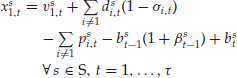
A generalized network investment model is presented in Figure 1. This figure depicts the flows across time for each of the asset classes. While all constraints cannot be put into a network model, the graphical form is easy for asset managers to comprehend. General linear and nonlinear programs are now readily available for solving the resulting problem. However, a network may have computational advantages for extremely large problems, such as security level models.
Figure 1 Network Representation for Each Scenario, ![]()

As with single-period models, the nonlinear objective function (1) can take several different forms. If the classical return-risk function is employed, then (1) becomes Max ![]() where Mean(wτ) is the expected total wealth and Risk(wτ) is the risk of the total wealth across the scenarios at the beginning of period τ. Parameter η indicates the relative importance of risk as compared with the expected value. This objective leads to an efficient frontier at period τ by allowing alternative values of η in the range [0,1]. It can be shown that a viable alternative to the mean-risk framework is the von Neumann-Morgenstern expected utility of wealth at the beginning of period τ.
where Mean(wτ) is the expected total wealth and Risk(wτ) is the risk of the total wealth across the scenarios at the beginning of period τ. Parameter η indicates the relative importance of risk as compared with the expected value. This objective leads to an efficient frontier at period τ by allowing alternative values of η in the range [0,1]. It can be shown that a viable alternative to the mean-risk framework is the von Neumann-Morgenstern expected utility of wealth at the beginning of period τ.
Let's review the six constraints:
The preceding constraints ensure that the scenarios with the same past will have identical decisions up to that period. While these constraints are numerous, solution algorithms take advantage of their simple structure. See Birge and Louveaux (1997), Dantzig and Infanger (1993), Kall and Wallace (1994), and Mulvey and Ruszczy![]() ski (1995), for example.
ski (1995), for example.
Figure 2 depicts the constraint structure for a split variable formulation of the stochastic asset allocation problem. This formulation has proven successful for solving the model using techniques such as the progressive hedging algorithm of Rockafellar and Wets (1991) and the DQA algorithm by Mulvey and Ruszczy![]() ski (1995). The split variable formulation can be beneficial for direct solvers that use the interior point method. Given today's powerful PCs, the nonlinear optimization system can be solved in a direct fashion for realistic-size implementations.
ski (1995). The split variable formulation can be beneficial for direct solvers that use the interior point method. Given today's powerful PCs, the nonlinear optimization system can be solved in a direct fashion for realistic-size implementations.
Figure 2 Split Variable Formulation (NAV: Nonanticipativity Variables, RV: Remaining Variables)

By substituting constraint (7) back into constraints (2) to (6), we obtain a standard form of the stochastic allocation problem. Constraints for this formulation exhibit a dual block diagonal structure for two-stage stochastic programs and a nested structure for general multistage problems. This formulation may be better for some direct solvers. The standard form of the stochastic program possesses fewer decision variables than the split variable model and is the preferred structure by many researchers in the field. This model can be solved by means of decomposition methods, for example, the L-shaped method (a specialization of Benders' algorithm). (See Birge and Louveaux, 1997; Consigli and Dempster, 1998; Dantzig and Infanger, 1993; and Kouwenberg and Zenios, 2006.)
As shown by Consigli and Dempster (1998), Dantzig and Infanger (1993), Mulvey et al. (2000), Ziemba and Mulvey (1998), and Ziemba (2003), a multistage model can provide superior performance over single-period models.
Modeling Future Uncertainties (Scenario Generation)
To model future uncertainty in our financial planning problem, we utilize a representative set of scenarios. In this section, we review the procedures for scenario generation and give details about the approach described.
In most cases, stochastic programming models require that the future uncertainties are approximated by a scenario tree with a finite number of states of the world at each time. The planning horizon is divided into T time periods (generally years for pension planning).
A sample scenario tree of three periods and nine scenarios is depicted in Figure 3. The root of the tree represents the current state of the world. A scenario is defined as a single branch from the root to any leaf of the tree (e.g., the boldfaced path corresponds to scenario 4). Thus, all of the parameter uncertainties are depicted along this branch. Each node represents a state of the world under a given scenario at a given time; for instance, the boldfaced node corresponds to the set of uncertainties at the end of period 2 under scenario 4. The stochastic program will determine an optimal decision for each node of the scenario tree, given the information available at that point. As there are multiple succeeding nodes, the optimal decisions will be determined without exploiting hindsight. A stochastic programming model will find the optimal policy that will fit the current state of the world and the decision maker in each node, while anticipating the optimal adjustment of the policy later on as the tree evolves and more information is revealed.
Figure 3 A Three-Period Scenario Tree

Generating scenario trees to represent the evolution of future uncertainty is a two-step process. Figure 4 depicts a diagram of the process.
Figure 4 From Historical Data to Scenario Trees
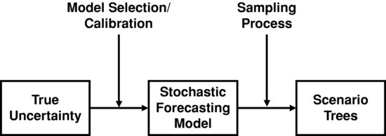
The first step involves the construction of a stochastic forecasting model. This involves choosing a model that would be appropriate for the uncertain variables and calibrating the parameters of this model using historical data.
The simplest approach, bootstrapping historical data, eliminates the need for a mathematical model (see, e.g., Grauer and Hakansson, 1982). Among mathematical models, stochastic differential equations and time series analysis are two commonly used techniques to generate anticipatory scenarios. Our preference is to employ the former technique, in which a sequence of economic factors (e.g., gross domestic product, corporate earnings, interest rates, and inflation) drive the state variables (see Mulvey [1996] for the details). The parameters of the SDEs for the economic factors and asset returns can be calibrated using historical data. A standard variance reduction method, antithetic variates, can be employed to improve the accuracy of the model's recommendations. Indirect inference methods for calibrating the parameters of the resulting stochastic system can be employed (see Gourieroux et al., 1993).
The next step involves the discretization of the scenarios generated by the stochastic forecasting model in the first step. To avoid any computational disadvantages, this has to be done using a small number of nodes, which in turn will lead to approximation errors. There are several methods to achieve this depending on the models employed in the first step (see Hoyland and Wallace, 2001; Kouwenberg and Zenios, 2006; Grebeck, Rachev, and Fabozzi, 2009; and Ziemba, 2003). We first create discretized sample paths by moment-matching, using the cascaded SDE structure in the first step. Then, we convert these sample paths to a scenario tree by clustering (see ![]() et al., 2002). We begin by grouping similar first stage values of the sample paths into clusters, and then continue sequentially through each stage.
et al., 2002). We begin by grouping similar first stage values of the sample paths into clusters, and then continue sequentially through each stage.
For an ALM system, one needs to generate scenarios for the liability side as well as the asset side. Obviously, both components are driven by economic factors. Liabilities are affected by actuarial predictions as well. When modeling the asset returns, one may need to use sentiment or expert judgment to improve the range of scenarios.
The future value of the liabilities can be especially tricky to project for institutions, such as pension plans, where the liabilities consist of several contracts and therefore the valuation is affected by various sources of uncertainty. For a typical pension plan, one can simulate the future status of the participants by making assumptions about the retirement rates, resignation frequency, promotion/demotion probabilities, and the mortality rate. Once this is done, the interest rates are forecasted and used to calculate the present value of the liabilities.
When modeling the asset returns, the economic factors that drive the primary asset-class returns are projected as a first step, which would then be followed by the projection of returns for these primary assets. More complex assets would be the last to be modeled in this setup. Alternatively, one can model all uncertain variables at once through one big set of multivariate time-series models.
KEY POINTS
- Stochastic programming is an operations research method for optimal decision making under uncertainty and bears suitable characteristics for modeling and solving financial planning applications, such as asset-liability management, capital budgeting, and fixed income portfolio management.
- The main features of a stochastic program are: random parameters with known (or partially known) distributions; several decision variables with many potential values; multiple discrete time periods for decisions; use of expectations (or other functions of decision variables) for objectives.
- Stochastic programs typically have larger problem size than stochastic control models, which put more emphasis on control rules and have more restrictive constraint assumptions.
- Stochastic programming models generally require that the future uncertainties are approximated by a scenario tree with a finite number of states of the world at each time.
- Multiperiod stochastic programs with a large number of parameters and scenarios result in large-scale deterministic-equivalent programs. Specialized software packages combined with algebraic modeling languages are utilized to efficiently tackle these problems.
REFERENCES
Beale, E. M. L. (1955). On minimizing a convex function subject to linear inequalities. Journal of Royal Statistical Society, Series B 17: 173–184.
Beltratti, A., Consiglio, A., and Zenios, S. A. (1999). Scenario modeling for the management of international bond portfolios. Annals of Operations Research 85: 227–247.
Benders, J. F. (1962). Partitioning procedures for solving mixed variables programming problems. Numerische Mathematik 4: 238–252.
Berger, A. J. (1995). Large Scale Stochastic Optimization with Applications to Finance. PhD Thesis, Princeton University.
Berger, A. J., Mulvey, J. M., and Ruszczy![]() ski, A. (1994). An extension of the DQA algorithm to convex stochastic programs. SIAM Journal on Optimization 4: 735–753.
ski, A. (1994). An extension of the DQA algorithm to convex stochastic programs. SIAM Journal on Optimization 4: 735–753.
Birge, J. R. (1985). Decomposition and partitioning methods for multistage stochastic linear programming. Operations Research 33: 989–1007.
Birge, J. R., Edirisinghe, N. C. P., and Ziemba, W. T. (eds.). (2002). Research in Stochastic Programming (Special Issue Annals of Operations Research). Baltzer Science Publishers BV.
Birge, J. R., and Louveaux, F. (1997). Introduction to Stochastic Programming. New York: Springer.
Black, F., and Scholes, M. (1973). The pricing of options and corporate liabilities. Journal of Political Economy 81: 637–654.
Bradley, S. P., and Crane, D. B. (1972). A dynamic model for bond portfolio management. Management Science 19, 2: 139–151.
Cariño, D. R., Kent, T., Myers, D. H., et al. (1994). The Russell-Yasuda Kasai model: An asset/liability model for a Japanese insurance company using multistage stochastic programming. Interfaces 24: 29–49.
Cariño, D. R., Myers, D. H., and Ziemba, W. T. (1998). Concepts, technical issues, and uses of the Russsell-Yasuda Kasai financial planning model. Operations Research 46: 450–462.
Cariño, D. R., and Ziemba, W. T. (1998). Formulation of the Russell-Yasuda Kasai financial planning model. Operations Research 46: 433–449.
Censor, Y., and Zenios, S. A. (1997). Optimization: Theory, Algorithms and Applications. Series on Numerical Mathematics and Scientific Computation. New York: Oxford University Press.
Charnes, A., and Cooper, W. W. (1959). Chance-constrained programming. Management Science 5: 73–79.
Cochrane, J. H. (2001). Asset Pricing. Princeton, NJ: Princeton University Press.
Consigli, G., and Dempster, M. A. H. (1998). Dynamic stochastic programming for asset-liability management. Annals of Operations Research 81: 131–161.
Constantinides, G. M. (1986). Capital market equilibrium with transaction costs. Journal of Political Economy 94: 842–862.
Dantzig, G. B. (1955). Linear programming under uncertainty. Management Science 1: 197–206.
Dantzig, G. B., and Infanger, G. (1993). Multistage stochastic linear programs for portfolio optimization. Annals of Operations Research 45: 59–76.
Dantzig, G. B., and Madansky, A. (1961). On the solution of two-stage linear programs under uncertainty. In Proceedings of the Fourth Berkeley Symposium on Mathematical Statistics and Probability. Berkeley: University of California Press.
De, K., Acharya, D., and Sahu, K. C. (1982). A chance-constrained goal programming model for capital budgeting. Journal of the Operational Research Society 33: 635–638.
Dumas, B., and Luciano, E. (1991). An exact solution to a dynamic portfolio choice problem under transaction costs. Journal of Finance 46: 577–595.
Dupačová, J., Hurt, J., and Stepan, J. (2002). Stochastic Modeling in Economics and Finance. Dordrecht, Netherlands: Kluwer Academic Publishers.
Ermoliev, Y., and Wets, R. J-B. (eds.). (1988). Numerical Methods for Stochastic Optimization. Berlin: Springer-Verlag.
Fishburn, P. C. (1977). Mean-variance risk analysis with risk associated with below target returns. American Economic Review 67: 116–126.
Fleten, S.-E., Hoyland, K., and Wallace, S. W. (2002). The performance of stochastic dynamic and fixed mix portfolio models. European Journal of Operational Research 140, 1: 37–49.
Geyer, A., and Ziemba, W. T. (2008). The Innovest Austrian pension fund financial planning model InnoALM. Operations Research 56: 797–810.
Golub B., Holmer, M., McKendall, R., Pohlman, L., and Zenios, S. A. (1995). A stochastic programming model for money management. European Journal of Operational Research 85: 282–296.
Gondzio, J., and Kouwenberg, R. (2001). High-performance computing for asset-liability management. Operations Research 49: 879–891.
Gourieroux, C., Monfort, A., and Renault, E. (1993). Indirect inference. Journal of Applied Econometrics 8: S85–S118.
Grauer, R. R., and Hakansson, N. H. (1982). Higher return, lower risk: Historical returns on long-run, actively managed portfolios of stocks, bonds and bills, 1936–78. Financial Analysts Journal 38: 39–53.
Granville, S., Pereira, M. V. F., and McCoy, M. (1994). Stochastic dual dynamic programming applied to financial planning problems. Technical Report PSR1, R-Alberto de Campos, Rio de Janeiro, Brazil.
Grebeck, M. J., Rachev, S.T., and Fabozzi, F. J. (2009). Stochastic programming and stable distributions in asset liability management. Journal of Risk 12, 2: 29–47.
Higle, J. L., and Sen, S. (1996). Stochastic Decomposition: A Statistical Method for Large Scale Stochastic Programming. Dordrecht, Netherlands: Kluwer Academic Publishers.
Hiller, R. S., and Eckstein, J. (1993). Stochastic dedication: Designing fixed income portfolios using massively parallel Benders decomposition. Management Science 39, 11: 1422–1438.
Holmer, M. R. (1994). The asset-liability management strategy system at Fannie Mae. Interfaces 24: 3–21.
Hoyland, K., and Wallace, S. (2001). Generating scenario trees for multistage problems. Management Science 47: 295–307.
Infanger, G. (1994). Planning under Uncertainty. Danvers, MA: Boyd and Fraser.
Kall, P., and Wallace, S. W. (1994). Stochastic Programming. New York: John Wiley & Sons.
Kallberg, J., White, R., and Ziemba, W. T. (1982). Short term financial planning under uncertainty. Management Science 28: 670–682.
Kouwenberg, R., and Zenios, S. A. (2006). Stochastic programming models for asset liability management. In S. A. Zenios and W. T. Ziemba (eds.), Handbook of Asset and Liability Management: Theory and Methodology (pp. 253–303). Amsterdam: North-Holland.
Kusy, M. I., and Ziemba, W. T. (1986). A bank asset and liability management model. Operations Research 34: 356–376.
Lockett, A. G., and Gear, A. E. (1975). Multistage capital budgeting under uncertainty. Journal of Financial and Quantitative Analysis 10, 1: 21–36.
Markowitz, H. M. (1952). Portfolio selection. Journal of Finance 7: 77–91.
Merton, R. C. (1969). Lifetime portfolio selection under uncertainty: The continuous time case. Review of Economics and Statistics 51: 247–257.
Merton, R. C. (1973). An intertemporal capital asset pricing model. Econometrica 41: 867–887.
Mulvey, J. M. (1989). A surplus optimization perspective. Investment Management Review 3: 31–39.
Mulvey, J. M. (1996). Generating scenarios for the Towers Perrin investment system. Interfaces 26: 1–15.
Mulvey, J. M., Gould, G., and Morgan, C. (2000). The asset and liability management system for Towers Perrin-Tillinghast. Interfaces 30: 96–114.
Mulvey, J. M., Rosenbaum, D. P., and Shetty, B. (1997). Strategic financial risk management and operations research. European Journal of Operational Research 97: 1–16.
Mulvey, J. M., and Ruszczy![]() ski, A. (1992). A diagonal quadratic approximation method for large scale linear programs. Operations Research Letters 12: 205–215.
ski, A. (1992). A diagonal quadratic approximation method for large scale linear programs. Operations Research Letters 12: 205–215.
Mulvey, J. M., and Ruszczy![]() ski, A. (1995). A new scenario decomposition method for large-scale stochastic optimization. Operations Research 43: 477–490.
ski, A. (1995). A new scenario decomposition method for large-scale stochastic optimization. Operations Research 43: 477–490.
Mulvey, J. M., and Simsek, K. D. (2002). Rebalancing strategies for long-term investors. In E. J. Kontoghiorghes, B. Rustem, and S. Siokos (eds.), Computational Methods in Decision-Making, Economics and Finance: Optimization Models (pp. 15–33). Netherlands: Kluwer Academic Publishers.
Mulvey, J. M., and Vladimirou, H. (1991). Solving multistage stochastic networks: An application of scenario aggregation. Networks 21: 619–643.
Mulvey, J. M., and Vladimirou, H. (1992). Stochastic network programming for financial planning problems. Management Science 38: 1642–1664.
Prékopa, A. (1995). Stochastic Programming. Dordrecht, Netherlands: Kluwer Academic Publishers.
Rockafellar, R. T., and Uryasev, S. (2000). Optimization of conditional Value-at-Risk. The Journal of Risk 2, 3: 21–41.
Rockafellar, R. T., and Wets, R. J-B. (1991). Scenario and policy aggregation in optimization under uncertainty. Mathematics of Operations Research 16: 119–147.
Ruszczy![]() ski, A., and Shapiro, A. (eds.). (2003). Stochastic programming. In Handbooks in Operations Research and Management Science, Volume 10. Amsterdam: North-Holland.
ski, A., and Shapiro, A. (eds.). (2003). Stochastic programming. In Handbooks in Operations Research and Management Science, Volume 10. Amsterdam: North-Holland.
Shreve, S. E., and Soner, H. M. (1991). Optimal investment and consumption with two bonds and transaction costs. Mathematical Finance 1: 53–84.
Turney, S. T. (1990). Deterministic and stochastic dynamic adjustment of capital investment budgets. Mathematical Computation and Modelling 13, 5: 1–9.
Van Slyke, R. M., and Wets, R. J-B. (1969). L-shaped linear programs with applications to optimal control and stochastic programming. SIAM Journal on Applied Mathematics 17: 638–663.
Wallace, S., Higle, J., and Sen, S. (eds.). (1996). Stochastic Programming, Algorithms and Models (Special Issue Annals of Operations Research). Baltzer Science Publishers BV.
Wallace, S. W., and Ziemba, W. T. (eds.). (2003). Applications of Stochastic Programming, SIAM Mathematical Series on Optimization.
Wets, R. J-B., and Ziemba, W. T. (eds.). (1999). Stochastic Programming—State of the Art (Special Issue Annals of Operations Research). Baltzer Science Publishers BV.
Worzel, K. J., Vassiadou-Zeniou, C., and Zenios, S. A. (1994). Integrated simulation and optimization models for tracking fixed-income indices. Operations Research 42: 223–233.
Zenios, S. A. (1992). Financial Optimization. Cambridge, UK: Cambridge University Press.
Zenios, S. A. (1995). Asset/liability management under uncertainty for fixed-income securities. Annals of Operations Research 59: 77–97.
Zenios, S. A., and Kang, P. (1993). Mean-absolute deviation and portfolio optimization for mortgage-backed securities. Annals of Operations Research 45: 433–450.
Zenios, S. A., and Ziemba, W. T. (2006). Handbook of Asset and Liability Management: Theory and Methodology. Amsterdam: North-Holland.
Ziemba, W. T. (2003). The Stochastic Programming Approach to Asset-Liability and Wealth Management. AIMR-Blackwell.
Ziemba, W. T., and Mulvey, J. (eds.). (1998). Worldwide Asset and Liability Modeling. Cambridge, UK: Cambridge University Press.
Ziemba, W. T., and Vickson, R. G. (1975). Stochastic Optimization Models in Finance. New York: Academic Press.