
Operational Risk Models
Identifying the core principles that underlie the operational risk process is the fundamental building block in deciding on the optimal model to be used. In this entry we provide an overview of models that have been put forward for the assessment of operational risk. These models are broadly classified into top-down models and bottom-up models.
Operational risk is distinct from credit risk and market risk, posing difficulties of implementation of the Basel II guidelines and strategic planning. We discuss some key aspects that distinguish operational risk from credit risk and market risk. They are related to the arrival process of loss events, the loss severity, and the dependence structure of operational losses across a bank's business units. Finally in this entry we reconsider the normality assumption—an assumption often made in modeling financial data—and question its applicability for the purpose of operational risk modeling.
OPERATIONAL RISK MODELS
Broadly speaking, operational risk models stem from two fundamentally different approaches: (1) the top-down approach, and (2) the bottom-up approach. Figure 1 illustrates a possible categorization of quantitative models.
Figure 1 Topology of Operational Risk Models

Top-down approaches quantify operational risk without attempting to identify the events or causes of losses.1 That is, the losses are simply measured on a macro basis. The principal advantage of this approach is that little effort is required with collecting data and evaluating operational risk. Bottom-up approaches quantify operational risk on a micro level being based on identified internal events, and this information is then incorporated into the overall capital charge calculation. The advantage of bottom-up approaches over top-down approaches lies in their ability to explain the mechanism of how and why operational risk is formed within an institution. Banks can either start with top-down models and use them as a temporary tool to estimate the capital charge and then slowly shift to the more advanced bottom-up models, or they can adopt bottom-up models from the start, provided that they have robust databases.
Models Based on Top-Down Approaches
In this section we will provide a brief look at the seven top-down approaches shown in Figure 1.2
Multifactor Equity Pricing Models
Multifactor equity pricing models, also referred to as multifactor models, can be utilized to perform a global analysis of banking risks and may be used for the purpose of integrated risk management, in particular for publicly traded firms. The stock return process Rt can be estimated by regressing stock return on a large number of external risk factor indexes It related to market risk, credit risks, and other nonoperational risks (such as interest rate fluctuations, stock price movements, and macroeconomic effects). Operational risk is then measured as the volatility of the residual term. Such models rely on the assumption that operational risk is the residual banking risk, after credit and market risks are accounted for.3
![]()
in which ![]() t is the residual term, a proxy for operational risk.
t is the residual term, a proxy for operational risk.
This approach relies on the widely known efficient market hypothesis that was introduced by Fama (1970), that states that in efficient capital markets all relevant past, publicly, and privately available information is reflected in current asset prices.
Capital Asset Pricing Model
Under the capital asset pricing model (CAPM) approach all risks are assumed to be measurable by the CAPM and represented by beta (β). CAPM, developed by Sharpe (1964), is an equilibrium model that describes the pricing of assets. It concludes that the expected security risk premium (i.e., expected return on security minus the risk-free rate of return) equals beta times the expected market risk premium (i.e., expected return on the market minus the risk-free rate of return).
Under the CAPM approach, operational risk is obtained by measuring market, credit, and other risks’ betas and deducting them from the total beta. With respect to applications to operational risk, the CAPM approach was discussed by Hiwatashi and Ashida (2002) and van den Brink (2002). According to van den Brink (2002), the CAPM approach has some limitations and so has not received a wide recognition for operational risk, but was in the past considered by Chase Manhattan Bank.
Income-Based Models
Income-based models resemble the multifactor equity price models: Operational risk is estimated as the residual variance by extracting market, credit, and other risks from the historical income (or earnings) volatility. Income-based models are described by Allen, Boudoukh, and Saunders (2004), who refer to these models as earnings at risk models and by Hiwatashi and Ashida (2002), who refer to them as the volatility approach. According to Cruz (2002), the profit and loss (P&L) volatility in a financial institution is attributed 50%, 15%, and 35% to credit risk, market risk, and operational and other risks, respectively.
Expense-Based Models
Expense-based models measure operational risk as fluctuations in historical expenses rather than income. The unexpected operational losses are captured by the volatility of direct expenses (as opposed to indirect expenses, such as opportunity costs, reputational risk, and strategic risk, that are outside the agreed scope of operational risk), adjusted for any structural changes within the bank.
Operating Leverage Models
Operating leverage models measure the relationship between operating expenses and total assets. Operating leverage is measured as a weighted combination of a fraction of fixed assets and a portion of operating expenses. Examples of calculating operating leverage amount per business line include taking 10% of fixed assets plus 25% times three months’ operating expenses for a particular business, or taking 2.5 times the monthly fixed expenses.4
Scenario Analysis and Stress Testing Models
Scenario analysis and stress testing models can be used for testing the robustness properties of loss models, in monetary terms, in the presence of potential events that are not part of banks’ actual internal databases. These models, also called expert judgment models by van den Brink (2002), are estimated based on the “what if” scenarios generated with reference to expert opinion, external data, catastrophic events that occurred in other banks, or imaginary high-magnitude events. Experts estimate the expected risk amounts and their associated probabilities of occurrence. For any particular bank, examples of scenarios include:5
- Bank's inability to reconcile a new settlement system with the original system.
- A class action suit alleging incomplete disclosure.
- Massive technology failure.
- High-scale unauthorized trading (for example, adding the total loss borne by the Barings bank preceding its collapse into the database, and reevaluating the model).
- Doubling the bank's maximum historical loss amount.
Additionally, stress tests can be used to see the likely increase in risk exposure due to removing a control or reduction in risk exposure due to tightening of controls.
Risk Indicator Models
Risk indicator models rely on a number (one or more) of operational risk exposure indicators to track operational risk. In the operational risk literature, risk indicator models are also called indicator approach models,6 risk profiling models,7 and peer-group comparison.8 A necessary aspect of such models is testing for possible correlations between risk factors. These models assume that there is a direct and significant relationship between the indicators and target variables. For example, Taylor and Hoffman (1999) illustrate how training expenditure has a reverse effect on the number of employee errors and customer complaints and Shih, Samad-Khan, and Medapa (2000) illustrate how a bank's size relates to the operational loss amount.
Risk indicator models may rely on a single indicator or multiple indicators. The former model is called the single-indicator approach;9 an example of such a model is the Basic Indicator Approach for quantification of the operational risk regulatory capital, proposed by the Basel II. The latter model is called the multi-indicator approach; an example of such a model is the Standardized Approach.
Models Based on Bottom-Up Approaches
An ideal internal operational risk assessment procedure would be to use a balanced approach, and include both top-down and bottom-up elements in the analysis.10 For example, scenario analysis can prove effective for backtesting purposes, and multifactor causal models are useful in performing operational Value-at-Risk (VaR) sensitivity analysis. Bottom-up approach models can be categorized into three groups:11 process-based models, actuarial-type models (or statistical models), and proprietary models.
Process-Based Models
There are three types of process-based models: (1) causal models and Bayesian belief networks, (2) reliability models, and (3) multifactor causal models. We describe each below.
The first group of process-based models is the causal models and Bayesian belief networks. Also called causal network models, causal models are subjective self-assessment models. Causal models form the basis of the scorecard models.12 These models split banking activities into simple steps; for each step, bank management evaluates the number of days needed to complete the step, the number of failures and errors, and so on, and then records the results in a “process map” (or scorecards) in order to identify potential weak points in the operational cycle. Constructing associated event trees that detect a sequence of actions or events that may lead to an operational loss is part of the analysis.13 For each step, bank management estimates a probability of its occurrence, called the subjective (or prior) probability. The ultimate event's probability is measured by the posterior probability. Prior and posterior probabilities can be estimated using the Bayesian belief networks.14 A variation of the causal models, connectivity models, focuses on the ex ante cause of operational loss event, rather than the ex post effect.
The second group of process-based models encompasses reliability models. These models are based on the frequency distribution of the operational loss events and their interarrival times. Reliability models focus on measuring the likelihood that a particular event will occur at some point or interval of time. We discuss this model below.
If f(t) is the density of a loss amount occurring at time t, then the reliability of the system is the probability of survival up to time t, denoted by R(t) and calculated as
![]()
The hazard rate (or the failure rate), h(t), is the rate at which losses occur per unit of time t, defined as
![]()
In practical applications, it is often convenient to use the Poisson-type arrival model to describe the occurrence of operational loss events. Under the simple Poisson model with the intensity rate λ (which represents the average number of events in any point of time), the interarrival times between the events (i.e., the time intervals between any two consecutive points of time in which an event takes place) follow an exponential distribution having density of form f(t) = λe−λt with mean interarrival time equal to 1/λ. The parameter λ is then the hazard rate for the simple Poisson process.
Finally, the third group of process-based models is multifactor causal models. These models can be used for performing the factor analysis of operational risk. These are regression-type models that examine the sensitivity of aggregate operational losses (or, alternatively, VaR) to various internal risk factors (or risk drivers). Multifactor causal models have been discussed in the VaR and operational risk literature.15 Examples of control factors include system downtime in minutes per day, number of employees in the back office, data quality (such as the ratio of the number of transactions with no input errors to the total number of transactions), total number of transactions, skill levels, product complexity, level of automation, customer satisfaction, and so on. Cruz (2002) suggests using manageable explanatory factors. In multifactor causal models, operational losses OR, or VaR, in a particular business unit at a point t, are regressed on a number of control factors:
![]()
where Xk, k = 1, 2,…, n, are the explanatory variables, and b's are the estimated coefficients. The model is forward-looking (or ex ante) as operational risk drivers are predictive of future losses. Extensions to the simple regression model may include autoregressive models, regime-switching models, ARMA/GARCH models, and others.
Actuarial Models
Actuarial models (or statistical models) are generally parametric statistical models. They have two key components: (1) the loss frequency and (2) the loss severity distributions of the historic operational loss data. Operational risk capital is measured by the VaR of the aggregated one-year losses.16
For the frequency of the loss data it is common to assume a Poisson process, with possible generalizations, such as a Cox process.
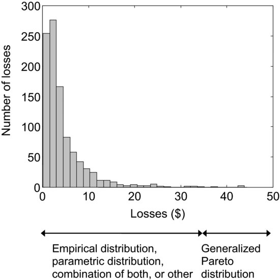
Actuarial models can differ by the type of the loss distribution. Empirical loss distribution models do not specify a particular class of loss distributions, but directly utilize the empirical distribution derived from the historic data. Parametric loss distribution models make use of a particular parametric distribution for the losses (or part of them), such as lognormal, Weibull, Pareto, and so on. Models based on extreme value theory (EVT) restrict attention to the tail events (i.e., the losses in the upper quantiles of the severity distribution), and VaR or other analyses are carried out upon fitting the generalized Pareto distribution to the data beyond a fixed high threshold. Van den Brink suggests using all three models simultaneously; Figure 2, inspired by his discussions, illustrates possible approaches. Yet another possibility is to fit an ARMA/GARCH model to the losses below a high threshold and the generalized Pareto distribution to the data exceeding it.
Figure 2 An Example of a Histogram of the Operational Loss Severity Distribution
Proprietary Models
Proprietary models for operational risk have been developed by major financial service companies and use a variety of bottom-up and top-down quantitative methodologies, as well as qualitative analysis, to evaluate operational risk. Banks can input their loss data into ready and systematized spreadsheets, which would be further categorized. The system then performs a qualitative and quantitative analysis of the data, and can carry out multiple tasks such as calculating regulatory capital, pooling internal data with external, performing Bayesian network analysis, and so on.
Specifics of Operational Loss Data
The nature of operational risk is very different from that of market risk and credit risk. In fact, operational losses share many similarities with insurance claims, suggesting that most actuarial models can be a natural choice of the model for operational risk, and models well developed by the insurance industry can be almost exactly applied to operational risk. In this section we discuss some key issues characterizing operational risk that must be taken into consideration before quantitative analysis is undertaken.
Scarcity of Available Historical Data
The major obstacle banks face in developing comprehensive models for operational risk is the scarcity of available historical operational loss data. As of 2011, generally, even the largest banks have no more than 11–12 years of loss data. Shortage of relevant data means that the models and conclusions drawn from the available limited samples would lack sufficient explanatory power. This in turn means that the estimates of the expected loss and VaR may be highly volatile and unreliable. In addition, complex statistical or econometric models cannot be tested on small samples.
The problem becomes amplified when dealing with modeling extremely high operational losses: One cannot model tail events when only a few such data are present in the internal loss database. Three solutions have been proposed: (1) pooling internal and external data, (2) supplementing actual losses with near-miss losses, and (3) scenario analysis and stress tests (discussed earlier in this entry).
The idea behind pooling internal and external data is to populate a bank's existing internal database with data from outside the bank. The rationale is twofold: (1) to expand the database and hence increase the accuracy of statistical estimations and (2) to account for losses that have not occurred within the bank but that are not completely improbable based on the histories of other banks. According to BIS,
… a bank's internal measurement system must reasonably estimate unexpected losses based on the combined use of internal and relevant external loss data… (BIS, 2006, p. 150)
Baud, Frachot, and Roncalli (2002) propose a statistical methodology to pool internal and external data. Their methodology accounts for the fact that external data are truncated from below (banks commonly report their loss data to external parties in excess of $1 million) and that bank size may be correlated with the magnitudes of losses. They showed that pooling internal and external data may help avoid underestimation of the capital charge.
Data Arrival Process
One of the difficulties that arise with modeling operational losses has to do with the irregular nature of the event arrival process. In market risk models, market positions are recorded on a frequent basis, many times daily depending on the entity, by marking to market. Price quotes are available daily or for those securities that are infrequently traded, model-based prices are available for marking a position to market. As for credit risk, credit ratings by rating agencies are available. In addition, rating agencies provide credit watches to identify credits that are candidates for downgrades. In contrast, operational losses occur at irregular time intervals suggesting a process of a discrete nature. This makes it similar to the reduced-form models for credit risk, in which the frequency of default (i.e., failure to meet a credit agreement) is of nontrivial concern. Hence, while in market risk we need to model only the return distribution in order to obtain VaR, in operational risk both loss severity and frequency distributions are important.
Another problem is related to timing and data recording issues. In market and credit risk models, the impact of a relevant event is almost immediately reflected in the market and credit returns. In an ideal scenario, banks would know how much of the operational loss would be borne by the bank from an event at the very moment the event takes place and would record the loss at this moment. However, from the practical point of view, this appears nearly impossible to implement, because it takes time for the losses to accumulate after an event takes place. Therefore, it may take days, months, or even years for the full impact of a particular loss event to be evaluated. Hence, there is the problem of discrepancy (i.e., a time lag) between the occurrence of an event and the time at which the incurred loss is being recorded.
This problem directly affects the method in which banks choose to record their operational loss data. When banks record their operational loss data, they record (1) the amount of loss, and (2) the corresponding date. We can identify three potential scenarios for the types of date banks might use:17
Depending on which of the three date types is used, the models for operational risk and conclusions drawn from them may be considerably different. For example, in the third case of accounting dates, we are likely to observe cyclicality/seasonal effects in the time series of the loss data (for example, many loss events would be recorded around the end of December), while in the first and second cases such effects are much less likely to be present in the data. Fortunately, however, selection of the frequency distribution does not have a serious impact on the resulting capital charge.18
Loss Severity Process
There are three main problems that operational risk analysts must be aware of with respect to the severity of operational loss data: (1) the nonnegative sign of the data, (2) the high degree of dispersion of the data, and (3) the shape of the data.
The first problem related to the loss severity data deals with the sign of the data. Depending on the movements in the interest or exchange rates, the oscillations in the market returns and indicators can take either a positive or negative sign. This is different in the credit and operational risk models—usually, only losses (i.e., negative cash flows) are assumed to take place.19 Hence, in modeling operational loss magnitudes, one should either consider fitting the loss distributions that are defined only on positive values, or should use distributions that are defined on negative and positive values, truncated at zero.
The second problem deals with the high degree of dispersion of loss data. Historical observations suggest that the movements in the market indicators are generally of relatively low magnitude. Bigger losses are usually attributed to credit risk. Finally, although most of the operational losses occur on a daily basis and hence are small in magnitude, the excessive losses of financial institutions are in general due to the operational losses, rather than credit or market risk–related losses. Empirical evidence indicates that there is an extremely high degree of dispersion of the operational loss magnitudes, ranging from near-zero to billions of dollars. In general, this dispersion is measured by variance or standard deviation.20
The third problem concerns the shape of the loss distribution. The shape of the data for operational risk is very different from that of market or credit risk. In market risk models, for example, the distribution of the market returns is often assumed to be nearly symmetric around zero. Asymmetric cases refer to the data whose distribution is either left-skewed (i.e., the left tail of the distribution is very long) or right-skewed (i.e., the right tail of the distribution is very long) and/or whose distribution has two or more peaks of different height. Operational losses are highly asymmetric, and empirical evidence on operational risk indicates that the losses are highly skewed to the right. This is in part explained by the presence of “low frequency/high severity” events. See Figure 2 for an exemplary histogram of operational losses.
As previously discussed, empirical evidence on operational losses indicates a majority of observations being located close to zero, and a small number of observations being of a very high magnitude. The first phenomenon refers to a high kurtosis (i.e., peak) of the data, and the second one indicates heavy tails (or fat tails). Distributions of such data are often described as leptokurtic.
The Gaussian (or normal) distribution is often used to model market risk and credit risk. It is characterized by two parameters, μ and σ, that are its mean and standard deviation. Figure 3 provides an example of a normal density. Despite being easy to work with and having attractive features (such as symmetry and stability under linear transformations), the Gaussian distribution makes several critical assumptions about the loss data. They include the following:
- The Gaussian assumption is useful for modeling the distribution of events that are symmetric around their mean. It has been empirically demonstrated that operational losses are not symmetric and severely right-skewed, meaning that the right tail of the loss distribution is very long.
- In most cases (except for the cases when the mean is very high), the use of Gaussian distribution allows for the occurrence of negative values. This is not a desirable property for modeling loss severity because negative losses are usually not possible.21
- More importantly, the Gaussian distribution has an exponential decay in its tails (this property puts the Gaussian distribution into the class of light-tailed distributions), which means that the tail events (i.e., the events of an unusually high or low magnitude) have a near-zero probability of occurrence. However, very high-magnitude operational losses can seriously jeopardize a financial institution. Thus, it would be inappropriate to model operational losses with a distribution that essentially excludes the possibility of high-impact individual losses. Empirical evidence strongly supports the conjecture that the distribution of operational losses is in fact very leptokurtic—that is, has a high peak and very heavy tails (i.e., very rare events are assigned a positive probability).
Figure 3 An Example of a Gaussian Density
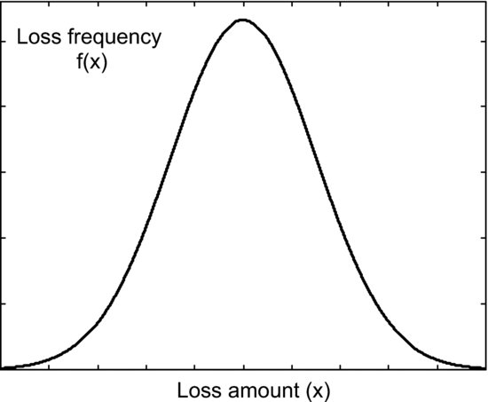
For the reasons presented above, it is unlikely that the Gaussian distribution would find much application for the assessment of operational risk.22 Heavier tailed distributions such as lognormal, Weibull, and even Pareto and alpha-stable, ought to be considered.
Dependence Between Business Units
In order to increase the accuracy of operational risk assessment, banks are advised to classify their operational loss data into groups of different degrees and nature of exposure to operational risk. Following this principle, the advanced measurement approaches (AMA) for the quantification of the operational risk capital charge, proposed by Basel II, suggest estimating operational risk capital separately for each “business line/event type” combination. Such a procedure is not common in market risk and credit risk models.
The most intuitive approach to combine risk measures collected from each of these “business line/event type” combinations is to add them up.23 However, such an approach may result in overestimation of the total capital charge because it implies a perfect positive correlation between groups. To prevent this from happening, it is essential to account for dependence between these combinations. Covariance and correlation are the simplest measures of dependency, but they assume a linear type of dependence, and therefore can produce misleading results if the linearity assumption is not true. An alternative approach would involve using copulas that are more flexible with respect to the form of the dependence structure that may exist between different groups. Another attractive property of copulas is their ability to capture the tail dependence between the distributions of random variables. Both properties are preserved under linear transformations of the variables.
KEY POINTS
- Operational risk measurement models are divided into top-down and bottom-up models.
- Top-down models use a macro-level regulatory approach to assess operational risk and determine the capital charge. They include multifactor equity price models, income and expense-based models, operating leverage models, scenario analysis and stress testing models, and risk indicator models.
- Bottom-up models originate from a micro-level analysis of a bank's loss data and consideration for the process and causes of loss events in determination of the capital charge. They include process-based models (such as causal network and Bayesian belief models, connectivity models, multifactor causal models, and reliability models), actuarial models, and proprietary models.
- Scarcity and reliability of available internal operational loss data remains a barrier preventing banks from developing comprehensive statistical models. Sufficiently large datasets are especially important for modeling low frequency high severity events. Three solutions have been put forward to help expand internal databases: pooling together internal and external data, accounting for near-misses, and stress tests.
- The nature of operational risk is fundamentally different from that of credit and market risks. Specifics of operational loss process include discrete data arrival process, delays between time of event and loss detection/accumulation, loss data taking only positive sign, high dispersion in magnitudes of loss data, distribution of loss data being severely right-skewed and heavy-tailed, and dependence between business units and event types.
- While many market and credit risk models make the convenient Gaussian assumption on the market returns or stock returns, this distribution is unlikely to be useful for the operational risk modeling because it is unable to capture the nonsymmetric and heavy-tailed nature of the loss data.
NOTES
1. An exception is the scenario analysis models in which specific events are identified and included in internal databases for stress testing. These events are, however, imaginable and do not appear in the banks’ original databases.
2. Some of these models are described in Allen, Boudoukh, and Saunders (2004).
3. See Chapter 2 in Chernobai, Rachev, and Fabozzi (2007) for an example of an empirical study that utilized such models in order to to evaluate the sensitivity of operational risk to macroeconomic factors.
4. See Marshall (2001).
5. The first four examples are due to Marshall (2001).
6. See Hiwatashi and Ashida (2002).
7. See Allen, Boudoukh, and Saunders (2004).
8. See van den Brink (2002).
9. See van den Brink (2002).
10. The Internal Measurement Approach (see description in BIS, 2001) combines some elements of the top-down approach and bottom-up approach: The gamma parameter in the formula for the capital charge is set externally by regulators, while the expected loss is determined based on internal data.
11. See Allen, Boudoukh, and Saunders (2004).
12. In February 2001 the Basel Committee suggested the Scorecard Approach as one possible advanced measurement approach to measure the operational risk capital charge.
13. See, for example, Marshall (2001) on the “fishbone analysis.”
14. Relevant Bayesian belief models with applications to operational risk are discussed in Alexander and Pezier (2001), Neil and Tranham (2002), and Giudici (2004), among others.
15. See also Haubenstock (2003) and Cruz (2002). The empirical study by Allen and Bali (2007) investigates the sensitivity of operational VaR to macroeconomic, rather than a bank's internal, risk factors.
16. Actuarial models form the basis of the loss distribution approach, an advanced measurement approach for operational risk. See BIS (2001).
17. Identification of the three types of dates are based on discussions with Marco Moscadelli (Banking Supervision Department, Bank of Italy).
18. See Carillo Menéndez (2005).
19. Certainly, it is possible that an event due to operational risk can incur unexpected profits for a bank, but usually this possibility is not considered.
20. Some very heavy-tailed distributions, such as the heavy-tailed Weibull, Pareto, or alpha-stable, can have an infinite variance. In these situations, robust measures of spread must be used.
21. Certainly, it is possible to use a truncated (at zero) version of the Gaussian distribution to fit operational losses.
22. Of course, a special case is fitting the Gaussian distribution to the natural logarithm of the loss data. This is equivalent (in terms of obtaining the maximum likelihood parameter estimates) to fitting the lognormal distribution to the original loss data.
23. This is the approach that was proposed in BIS (2001).
REFERENCES
Alexander, C. and Pezier, J. (2001). Taking control of operational risk. Futures and Options World 366: 60–65.
Allen, L. and Bali, T. (2007). Cyclicality in catastrophic and operational risk measurements. Journal of Banking and Finance 31, 4: 1191–1235.
Allen, L., Boudoukh, J., and Saunders, A. (2004). Understanding Market, Credit, and Operational Risk: The Value-at-Risk Approach. Oxford: Blackwell Publishing.
Baud, N., Frachot, A., and Roncalli, T. (2002). Internal data, external data, and consortium data for operational risk measurement: How to pool data properly? Technical report, Groupe de Recherche Opérationelle, Crédit Lyonnais, France.
Bank for International Settlements (2001). Consultative document: Operational risk. http://www.bis.org.
Bank for International Settlements (2006). International convergence of capital measurement and capital standards. http://www.bis.org.
Carillo Menéndez, S. (2005). Operational risk. Presentation at International Summer School on Risk Measurement and Control, Rome, June 2005.
Chernobai, A., Rachev, S. T., and Fabozzi, F. J. (2007). Operational Risk: A Guide to Basel II Capital Requirements, Models, and Analysis. Hoboken, NJ: John Wiley & Sons.
Cruz, M. G. (2002). Modeling, Measuring, and Hedging Operational Risk. Chichester, NY: John Wiley & Sons.
Fama, E. F. (1970). Efficient capital markets: A review of theory and empirical work. Journal of Finance 25: 383–417.
Giudici, P. (2004), Integration of qualitative and quantitative operational risk data: A Bayesian approach. In M. G. Cruz (ed.), Operational Risk Modelling and Analysis. Theory and Practice. London: RISK Books.
Haubenstock, M. (2003). The operational risk management framework. In C. Alexander (ed.), Operational Risk: Regulation, Analysis, and Management. London: Prentice Hall.
Hiwatashi, J., and Ashida, H. (2002). Advancing operational risk management using Japanese banking experiences. Technical report, Federal Reserve Bank of Chicago.
Marshall, C. L. (2001). Measuring and Managing Operational Risk in Financial Institutions: Tools, Techniques, and Other Resources. Chichester, NY: John Wiley & Sons.
Neil, M., and Tranham, E. (2002). Using Bayesian networks to predict op risk. Operational Risk, August: 8–9.
Sharpe, W. F. (1964). Capital asset prices: A theory of market equilibrium under conditions of risk. Journal of Finance 19: 425–442.
Shih, J., Samad-Khan, A. J., and Medapa, P. (2000). Is the size of an operational risk related to firm size? Operational Risk, January.
Taylor, D., and Hoffman, D. (1999). How to avoid signal failure. Risk, November: 13–15.
van den Brink, J. (2002). Operational Risk: The New Challenge for Banks. New York: Palgrave.