
Pricing of Futures/Forwards and Options
Derivative instruments play an important role in financial markets as well as commodity markets by allowing market participants to control their exposure to different types of risk. When using derivatives, a market participant should understand the basic principles of how they are valued. While there are many models that have been proposed for valuing financial instruments that trade in the cash (spot) market, the valuation of all derivative models is based on arbitrage arguments. Basically, this involves developing a strategy or a trade wherein a package consisting of a position in the underlying (that is, the underlying asset or instrument for the derivative contract) and borrowing or lending so as to generate the same cash flow profile as the derivative. The value of the package is then equal to the theoretical price of the derivative. If the market price of the derivative deviates from the theoretical price, then the actions of arbitrageurs will drive the market price of the derivative toward its theoretical price until the arbitrage opportunity is eliminated.
In developing a strategy to capture any mispricing, certain assumptions are made. When these assumptions are not satisfied in the real world, the theoretical price can only be approximated. Moreover, a close examination of the underlying assumptions necessary to derive the theoretical price indicates how a pricing formula must be modified to value specific contracts.
In this entry, how futures, forwards, and options are valued is explained. The valuation of other derivatives such as swaps, caps, and floors is described in other entries.
PRICING OF FUTURES/FORWARD CONTRACTS
The pricing of futures and forward contracts is similar. If the underlying asset for both contracts is the same, the difference in pricing is due to differences in features of the contract that must be dealt with by the pricing model. To understand the differences, we begin with a definition of the two contracts.
A futures contract and a forward contract are agreements between a buyer and a seller, in which the buyer agrees to take delivery of the underlying at a specified price at some future date and the seller agrees to make delivery of the underlying at the specified price at the same future date. The buyer and the seller of the contract refers to the obligation that the party has in the future since neither party is obligated to transact in the underlying at the time of the trade. The futures price in the case of a futures contract or forward price in the case of a forward contract is the price at which the parties have agreed to transact in the future. The settlement date or delivery date is the future date when the two parties have agreed to transact (that is, buy or sell the underlying).
Differences between Futures and Forward Contracts
Futures contracts are standardized agreements as to the delivery date (or month) and quality of the deliverable, and are traded on organized exchanges. Associated with every futures exchange is a clearinghouse. The clearinghouse plays an important function: It guarantees that both parties to the trade will perform in the future. In the absence of a clearinghouse, the risk that the two parties face is that in the future when both parties are obligated to perform one of the parties will default. This risk faced in any derivative contract is referred to as counterparty risk. The clearinghouse allows the two parties to enter into a trade without worrying about counterparty risk with respect to the counterparty to the trade. The reason is that after the trade is executed by the parties, the relationship between the two parties is terminated. The clearinghouse interposes itself as the buyer for every sale and the seller for every purchase. Consequently, the two parties to the trade are free to liquidate their positions without involving the original counterparty.
To protect itself against the counterparty risk of both the buyer and seller to the trade, the exchange where the contract is traded requires that when a position is first taken in a futures contract, both parties must deposit a minimum dollar amount per contract. This amount is specified by the exchange and referred to as initial margin. The parties have a choice of providing the initial margin in the form of cash or an interest-bearing security such as a Treasury bill. As the price of the futures contract fluctuates each trading day, the value of the equity of each party in the position changes. The equity in a futures margin account is measured by the sum of all margins posted and all daily gains less all daily losses to the account. To further protect itself against counterparty risk, the exchange specifies that the parties satisfy minimum equity positions. Maintenance margin is the minimum level that the exchange specifies that a party's equity position may fall as a result of an unfavorable price movement before a party is required to deposit additional margin. Variation margin is the additional margin that a party is required to provide in order to bring the equity in the margin account back to its initial margin level. If a party fails to furnish variation margin within 24 hours, the exchange closes the futures position out. Unlike initial margin, variation margin must be in cash rather than an interest-bearing security. Any excess margin in a party's margin account may be withdrawn.
In pricing futures contracts, the potential interim cash flows of futures contracts that are due to variation margin, in the case of adverse price movements, or withdrawal of cash for a party that experiences a favorable price movement that results in the margin account's having excess margin must be taken into account.
We'll now compare these characteristics of a futures contract to a forward contact. A forward contract is an over-the-counter (OTC) instrument. That is, it is not an exchange-traded product. A forward contract is usually nonstandardized because the terms of each contract are negotiated individually between the parties to the trade. Also, there is no clearinghouse for trading forward contracts, and secondary markets are often nonexistent or extremely thin.
As just explained, futures contracts are marked to market at the end of each trading day. A forward contract may or may not be marked to market, depending on the wishes of the two parties. For example, both parties to a forward contract may be high-credit-quality entities. The parties may feel comfortable with the counterparty risk up to some specified amount and not require margin. Or one party may be satisfied with the high quality of the counterparty but the other party may not. In such cases, the forward contract may call for the marking to market of the position of only one of the counterparties. For a forward contract that is not marked to market, there are no interim cash-flow effects because no additional margin is required.
Other than these differences, which reflect the institutional arrangements in the two markets, most of what we say about the pricing of futures contracts applies equally to the pricing of forward contracts.
Basic Futures Pricing Model
We will illustrate the basic model for pricing futures contracts here. By “basic” we mean that we are extrapolating from the nuisances of the underlying for a specific contract. The issues associated with applying the basic pricing model to some of the more popular futures contracts are described in other entries. Moreover, while the model described here is said to be a model for pricing futures, technically, it is a model for pricing forward contracts with no mark-to-market requirements.
Rather than deriving the formula algebraically, the basic pricing model will be demonstrated using an illustration. We make the following six assumptions for a futures contract that has no initial and variation margin and which the underlying is asset U:
The objective is to determine what the futures price of this contract should be. To do so, suppose that the futures price in the market is $105. Let's see if that is the correct price. We can check this by implementing the following simple strategy:
- Sell the futures contract at $105.
- Purchase asset U in the cash market for $100.
- Borrow $100 for three months at 4% per year ($1 per quarter).
The purchase of asset U is accomplished with the borrowed funds. Hence, this strategy does not involve any initial cash outlay. At the end of three months, the following occurs
- $2 is received from holding asset U.
- Asset U is delivered to settle the futures contract.
- The loan is repaid.
This strategy results in the following outcome:
From settlement of the futures contract:
| Proceeds from sale of asset U to settle | |
| the futures contract | = $105 |
| Payment received from investing in | |
| asset U for three months | =2 |
| Total proceeds | = $107 |
From the loan:
| Repayment of principal of loan | = $100 |
| Interest on loan (1% for three months) | =1 |
| Total outlay | = $101 |
| Profit from the strategy | = $6 |
The profit of $6 from this strategy is guaranteed regardless of what the cash price of asset U is three months from now. This is because in the preceding analysis of the outcome of the strategy, the cash price of asset U three months from now never enters the analysis. Moreover, this profit is generated with no investment outlay; the funds needed to acquire asset U are borrowed when the strategy is executed. In financial terms, the profit in the strategy we have just illustrated arises from a riskless arbitrage between the price of asset U in the cash market and the price of asset U in the futures market.
In a well-functioning market, arbitrageurs who could realize this riskless profit for a zero investment would implement the strategy described above. By selling the futures and buying asset U in order to implement the strategy, this would force the futures price down so that at some price for the futures contract, the arbitrage profit is eliminated.
This strategy that resulted in the capturing of the arbitrage profit is referred to as a cash-and-carry trade. The reason for this name is that implementation of the strategy involves borrowing cash to purchase the underlying and “carrying” that underlying to the settlement date of the futures contract.
From the cash-and-carry trade we see that the futures price cannot be $105. Suppose instead that the futures price is $95 rather than $105. Let's try the following strategy to see if that price can be sustained in the market:
- Buy the futures contract at $95.
- Sell (short) asset U for $100.
- Invest (lend) $100 for three months at 1% per year.
We assume once again that in this strategy that there is no initial margin and variation margin for the futures contract. In addition, we assume that there is no cost to selling the asset short and lending the money. Given these assumptions, there is no initial cash outlay for the strategy just as with the cash-and-carry trade. Three months from now,
- Asset U is purchased to settle the long position in the futures contract.
- Asset U is accepted for delivery.
- Asset U is used to cover the short position in the cash market.
- Payment is made of $2 to the lender of asset U as compensation for the quarterly payment.
- Payment is received from the borrower of the loan of $101 for principal and interest.
More specifically, the strategy produces the following at the end of three months:
From settlement of the futures contract:
| Price paid for purchase of asset U to | |
| settle futures contract | = $95 |
| Proceeds to lender of asset U to borrow | |
| the asset | =2 |
| Total outlay | = $97 |
From the loan:
| Principal from loan | = $100 |
| Interest earned on loan ($1 for three months) | =1 |
| Total proceeds | = $101 |
| Profit from the strategy | = $4 |
As with the cash and trade, the $4 profit from this strategy is a riskless arbitrage profit. This strategy requires no initial cash outlay, but will generate a profit whatever the price of asset U is in the cash market at the settlement date. In real-world markets, this opportunity would lead arbitrageurs to buy the futures contract and short asset U. The implementation of this strategy would be to raise the futures price until the arbitrage profit disappeared.
This strategy that is implemented to capture the arbitrage profit is known as a reverse cash-and-carry trade. That is, with this strategy, the underlying is sold short and the proceeds received from the short sale are invested.
We can see that the futures price cannot be $95 or $105. What is the theoretical futures price given the assumptions in our illustration? It can be shown that if the futures price is $99 there is no opportunity for an arbitrage profit. That is, neither the cash-and-carry trade nor the reverse cash-and-carry trade will generate an arbitrage profit.
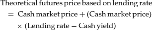
In general, the formula for determining the theoretical futures price given the assumptions of the model is:

In the formula given by (1), “Financing cost” is the interest rate to borrow funds and “Cash yield” is the payment received from investing in the asset as a percentage of the cash price. In our illustration, the financing cost is 1% and the cash yield is 2%.
In our illustration, since the cash price of asset U is $100, the theoretical futures price is:
![]()
The future price can be above or below the cash price depending on the difference between the financing cost and cash yield. The difference between these rates is called the net financing cost. A more commonly used term for the net financing cost is the cost of carry, or simply, carry. Positive carry means that the cash yield exceeds the financing cost. (Note that while the difference between the financing cost and the cash yield is a negative value, carry is said to be positive.) Negative carry means that the financing cost exceeds the cash yield. Below is a summary of the effect of carry on the difference between the futures price and the cash market price:
| Positive carry | Futures price will sell at a discount to cash price. |
| Negative carry | Futures price will sell at a premium to cash price. |
| Zero | Futures price will be equal to the cash price. |
Note that at the settlement date of the futures contract, the futures price must equal the cash market price. The reason is that a futures contract with no time left until delivery is equivalent to a cash market transaction. Thus, as the delivery date approaches, the futures price will converge to the cash market price. This fact is evident from the formula for the theoretical futures price given by (1). The financing cost approaches zero as the delivery date approaches. Similarly, the yield that can be earned by holding the underlying approaches zero. Hence, the cost of carry approaches zero, and the futures price approaches the cash market price.
A Closer Look at the Theoretical Futures Price
In deriving theoretical futures price using the arbitrage argument, several assumptions had to be made. These assumptions as well as the differences in contract specifications will result in the futures price in the market deviating from the theoretical futures price as given by (1). It may be possible to incorporate these institutional and contract specification differences into the formula for the theoretical futures price. In general, however, because it is oftentimes too difficult to allow for these differences in building a model for the theoretical futures price, the end result is that one can develop bands or boundaries for the theoretical futures price. So long as the futures price in the market remains within the band, no arbitrage opportunity is possible.
Next, we will look at some of the institutional and contract specification differences that cause prices to deviate from the theoretical futures price as given by the basic pricing model.
Interim Cash Flows
In the derivation of a basic pricing model, it is assumed that no interim cash flows arise because of changes in futures prices (that is, there is no variation margin). As noted earlier, in the absence of initial and variation margins, the theoretical price for the contract is technically the theoretical price for a forward contract that is not marked to market rather than a futures contract.
In addition, the model assumes implicitly that any dividends or coupon interest payments are paid at the settlement date of the futures contract rather than at any time between initiation of the cash position and settlement of the futures contract. However, we know that interim cash flows for the underlying for financial futures contracts do have interim cash flows. Consider stock index futures contracts and bond futures contracts.
For a stock index, there are interim cash flows. In fact, there are many cash flows that are dependent upon the dividend dates of the component companies. To correctly price a stock index future contract, it is necessary to incorporate the interim dividend payments. Yet, the dividend rate and the pattern of dividend payments are not known with certainty. Consequently, they must be projected from the historical dividend payments of the companies in the index. Once the dividend payments are projected, they can be incorporated into the pricing model. The only problem is that the value of the dividend payments at the settlement date will depend on the interest rate at which the dividend payments can be reinvested from the time they are projected to be received until the settlement date. The lower the dividend, and the closer the dividend payments to the settlement date of the futures contract, the less important the reinvestment income is in determining the futures price.
In the case of a Treasury futures contract, the underlying is a Treasury note or a Treasury bond. Unlike a stock index futures contract, the timing of the interest payments that will be made by the U.S. Department of the Treasury for a given issue that is acceptable as deliverable for a contract is known with certainty and can be incorporated into the pricing model. However, the reinvestment interest that can be earned from the payment dates to the settlement of the contract is unknown and depends on prevailing interest rates at each payment date.
Differences in Borrowing and Lending Rates
In the formula for the theoretical futures price, it is assumed in the cash-and-carry trade and the reverse cash-and-carry trade that the borrowing rate and lending rate are equal. Typically, however, the borrowing rate is higher than the lending rate. The impact of this inequality is important and easy to quantify.
In the cash-and-carry trade, the theoretical futures price as given by (1) becomes:

For the reverse cash-and-carry trade, it becomes
Formulas (2) and (3) together provide a band between which the actual futures price can exist without allowing for an arbitrage profit. Equation (2) establishes the upper value for the band while equation (3) provides the lower value for the band. For example, assume that the borrowing rate is 6% per year, or 1.5% for three months, while the lending rate is 4% per year, or 1% for three months. Using equation (2), the upper value for the theoretical futures price is $99.5 and using equation (3) the lower value for the theoretical futures price is $99.
Transaction Costs
The two strategies to exploit any price discrepancies between the cash market and theoretical price for the futures contract will require the arbitrageur to incur transaction costs. In real-world financial markets, the costs of entering into and closing the cash position as well as round-trip transaction costs for the futures contract affect the futures price. As in the case of differential borrowing and lending rates, transaction costs widen the bands for the theoretical futures price.
Short Selling
The reverse cash-and-strategy trade requires the short selling of the underlying. It is assumed in this strategy that the proceeds from the short sale are received and reinvested. In practice, for individual investors, the proceeds are not received, and, in fact, the individual investor is required to deposit margin (securities margin and not futures margin) to short sell. For institutional investors, the underlying may be borrowed, but there is a cost to borrowing. This cost of borrowing can be incorporated into the model by reducing the cash yield on the underlying. For strategies applied to stock index futures, a short sale of the components stocks in the index means that all stocks in the index must be sold simultaneously. This may be difficult to do and therefore would widen the band for the theoretical future price.
Known Deliverable Asset and Settlement Date
In the two strategies to arbitrage discrepancies between the theoretical futures price and the cash market price, it is assumed that (1) only one asset is deliverable and (2) the settlement date occurs at a known, fixed point in the future. Neither assumption is consistent with the delivery rules for some futures contracts. For U.S. Treasury note and bond futures contracts, for example, the contract specifies that any one of several Treasury issues that is acceptable for delivery can be delivered to satisfy the contract. Such issues are referred to as deliverable issues. The selection of which deliverable issue to deliver is an option granted to the party who is short the contract (that is, the seller). Hence, the party that is long the contract (that is, the buyer of the contract) does not know the specific Treasury issue that will be delivered. However, market participants can determine the cheapest-to-deliver issue from the issues that are acceptable for delivery. It is this issue that is used in obtaining the theoretical futures price. The net effect of the short's option to select the issue to deliver to satisfy the contract is that it reduces the theoretical future price by an amount equal to the value of the delivery option granted to the short.
Moreover, unlike other futures contracts, the Treasury bond and note contracts do not have a delivery date. Instead, there is a delivery month. The short has the right to select when in the delivery month to make delivery. The effect of this option granted to the short is once again to reduce the theoretical futures price below that given by equation (1). More specifically,
(4)
Deliverable as a Basket of Securities
Some futures contracts have as the underlying a basket of assets or an index. Stock index futures are the most obvious example. At one time, municipal futures contracts were actively traded and the underlying was a basket of municipal securities. The problem in arbitraging futures contracts in which there is a basket of assets or an index is that it may be too expensive to buy or sell every asset included in the basket or index. Instead, a portfolio containing a smaller number of assets may be constructed to track the basket or index (which means having price movements that are very similar to changes in the basket or index). Nonetheless, the two arbitrage strategies involve a tracking portfolio rather than a single asset for the underlying, and the strategies are no longer risk-free because of the risk that the tracking portfolio will not precisely replicate the performance of the basket or index. For this reason, the market price of futures contracts based on baskets of assets or an index is likely to diverge from the theoretical price and have wider bands.
Different Tax Treatment of Cash and Futures Transaction
Participants in the financial market cannot ignore the impact of taxes on a trade. The strategies that are implemented to exploit arbitrage opportunities between prices in the cash and futures markets and the resulting pricing model must recognize that there are differences in the tax treatment under the tax code for cash and futures transactions. The impact of taxes must be incorporated into the pricing model.
PRICING OF OPTIONS
Now we will look at the basic principles for valuing options. There are two parties to an option contract: the buyer and the writer or seller. The writer of the option grants the buyer of the option the right, but not the obligation, to either purchase from or sell to the writer something at a specified price within a specified period of time (or at a specified date). In exchange for the right that the writer grants the buyer, the buyer pays the writer a certain sum of money. This sum is called the option price or option premium. The price at which the underlying may be purchased or sold is called the exercise price or strike price. The option's expiration date (or maturity date) is the last date at which the option buyer can exercise the option. After the expiration date, the contract is void and has no value.
There are two types of options: call options and put options. A call option, or simply call, is one in which the option writer grants the buyer the right to purchase the underlying. When the option writer grants the buyer the right to sell the underlying, the option is called a put option, or simply, a put.
The timing of the possible exercise of an option is an important characteristic of an option contract. An American option allows the option buyer to exercise the option at any time up to and including the expiration date. A European option allows the option buyer to exercise the option only on the expiration date.
As with futures and forward contracts, the theoretical price of an option is also derived based on arbitrage arguments. However, as will be explained, the pricing of options is not as simple as the pricing of futures and forward contracts.
Basic Components of the Option Price
The theoretical price of an option is made up of two components: the intrinsic value and a premium over intrinsic value.
Intrinsic Value
The intrinsic value is the option's economic value if it is exercised immediately. If no positive economic value would result from exercising immediately, the intrinsic value is zero. An option's intrinsic value is easy to compute given the price of the underlying and the strike price.
For a call option, the intrinsic value is the difference between the current market price of the underlying and the strike price. If that difference is positive, then the intrinsic value equals that difference; if the difference is zero or negative, then the intrinsic value is equal to zero. For example, if the strike price for a call option is $100 and the current price of the underlying is $109, the intrinsic value is $9. That is, an option buyer exercising the option and simultaneously selling the underlying would realize $109 from the sale of the underlying, which would be covered by acquiring the underlying from the option writer for $100, thereby netting a $9 gain.
An option that has a positive intrinsic value is said to be in-the-money. When the strike price of a call option exceeds the underlying's market price, it has no intrinsic value and is said to be out-of-the-money. An option for which the strike price is equal to the underlying's market price is said to be at-the-money. Both at-the-money and out-of-the-money options have intrinsic values of zero because it is not profitable to exercise them. Our call option with a strike price of $100 would be (1) in the money when the market price of the underlying is more than $100; (2) out of the money when the market price of the underlying is less than $100, and (3) at the money when the market price of the underlying is equal to $100.
For a put option, the intrinsic value is equal to the amount by which the underlying's market price is below the strike price. For example, if the strike price of a put option is $100 and the market price of the underlying is $95, the intrinsic value is $5. That is, the buyer of the put option who simultaneously buys the underlying and exercises the put option will net $5 by exercising. The underlying will be sold to the writer for $100 and purchased in the market for $95. With a strike price of $100, the put option would be (1) in the money when the underlying's market price is less than $100, (2) out of the money when the underlying's market price exceeds $100, and (3) at the money when the underlying's market price is equal to $100.
Time Premium
The time premium of an option, also referred to as the time value of the option, is the amount by which the option's market price exceeds its intrinsic value. It is the expectation of the option buyer that at some time prior to the expiration date changes in the market price of the underlying will increase the value of the rights conveyed by the option. Because of this expectation, the option buyer is willing to pay a premium above the intrinsic value. For example, if the price of a call option with a strike price of $100 is $12 when the underlying's market price is $104, the time premium of this option is $8 ($12 minus its intrinsic value of $4). Had the underlying's market price been $95 instead of $104, then the time premium of this option would be the entire $12 because the option has no intrinsic value. All other things being equal, the time premium of an option will increase with the amount of time remaining to expiration.
An option buyer has two ways to realize the value of an option position. The first way is by exercising the option. The second way is to sell the option in the market. In the first example above, selling the call for $12 is preferable to exercising, because the exercise will realize only $4 (the intrinsic value), but the sale will realize $12. As this example shows, exercise causes the immediate loss of any time premium. It is important to note that there are circumstances under which an option may be exercised prior to the expiration date. These circumstances depend on whether the total proceeds at the expiration date would be greater by holding the option or exercising and reinvesting any received cash proceeds until the expiration date.
Put–Call Parity Relationship
For a European put and a European call option with the same underlying, strike price, and expiration date, there is a relationship between the price of a call option, the price of a put option, the price of the underlying, and the strike price. This relationship is known as the put–call parity relationship. The relationship is:

Factors That Influence the Option Price
The factors that affect the price of an option include the:
- Market price of the underlying.
- Strike price of the option.
- Time to expiration of the option.
- Expected volatility of the underlying over the life of the option.
- Short-term, risk-free interest rate over the life of the option.
- Anticipated cash payments on the underlying over the life of the option.
The impact of each of these factors may depend on whether (1) the option is a call or a put, and (2) the option is an American option or a European option. Table 1 summarizes how each of the six factors listed above affects the price of a put and call option. Here, we briefly explain why the factors have the particular effects.
Table 1 Summary of Factors That Affect the Price of an Option
| Effect of an Increase of Factor On | ||
| Factor | Call Price | Put Price |
| Market price of underlying | Increase | Decrease |
| Strike price | Decrease | Increase |
| Time to expiration of option | Increase | Increase |
| Expected volatility | Increase | Increase |
| Short-term, risk-free interest rate | Increase | Decrease |
| Anticipated cash payments | Decrease | Increase |
Market Price of the Underlying Asset
The option price will change as the price of the underlying changes. For a call option, as the underlying's price increases (all other factors being constant), the option price increases. The opposite holds for a put option: As the price of the underlying increases, the price of a put option decreases.
Strike Price
The strike price is fixed for the life of the option. All other factors being equal, the lower the strike price, the higher the price for a call option. For put options, the higher the strike price, the higher the option price.
Time to Expiration of the Option
After the expiration date, an option has no value. All other factors being equal, the longer the time to expiration of the option, the higher the option price. This is because, as the time to expiration decreases, less time remains for the underlying's price to rise (for a call buyer) or fall (for a put buyer), and therefore the probability of a favorable price movement decreases. Consequently, as the time remaining until expiration decreases, the option price approaches its intrinsic value.
Expected Volatility of the Underlying over the Life of the Option
All other factors being equal, the greater the expected volatility (as measured by the standard deviation or variance) of the underlying, the more the option buyer would be willing to pay for the option, and the more an option writer would demand for it. This occurs because the greater the expected volatility, the greater the probability that the movement of the underlying will change so as to benefit the option buyer at some time before expiration.
Short-Term, Risk-Free Interest Rate over the Life of the Option
Buying the underlying requires an investment of funds. Buying an option on the same quantity of the underlying makes the difference between the underlying's price and the option price available for investment at an interest rate at least as high as the risk-free rate. Consequently, all other factors being constant, the higher the short-term, risk-free interest rate, the greater the cost of buying the underlying and carrying it to the expiration date of the call option. Hence, the higher the short-term, risk-free interest rate, the more attractive the call option will be relative to the direct purchase of the underlying. As a result, the higher the short-term, risk-free interest rate, the greater the price of a call option.
Anticipated Cash Payments on the Underlying over the Life of the Option
Cash payments on the underlying tend to decrease the price of a call option because the cash payments make it more attractive to hold the underlying than to hold the option. For put options, cash payments on the underlying tend to increase the price.
Option Pricing Models
Earlier in this entry, it was explained how the theoretical price of a futures contract and forward contract can be determined on the basis of arbitrage arguments. An option pricing model uses a set of assumptions and arbitrage arguments to derive a theoretical price for an option. Deriving a theoretical option price is much more complicated than deriving a theoretical futures or forward price because the option price depends on the expected volatility of the underlying over the life of the option.
Several models have been developed to determine the theoretical price of an option. The most popular one was developed by Fischer Black and Myron Scholes (1973) for valuing European call options on common stock. The Black-Scholes model requires as input the six factors discussed above that affect the value of an option. Several modifications to the Black-Scholes model followed. One such model is the lattice model suggested by Cox, Ross, and Rubinstein (1979), Rendleman and Bartter (1979), and Sharpe (1981).
Basically, the idea behind the arbitrage argument is that if the payoff from owning a call option can be replicated by (1) purchasing the underlying for the call option and (2) borrowing funds to purchase the underlying, then the cost of creating the replicating strategy (position) is the theoretical price of the option.
KEY POINTS
- For futures and forward contracts, the theoretical price can be derived using arbitrage arguments. Specifically, a cash-and-carry trade can be implemented to capture the arbitrage profit for an overpriced futures or forward contract while a reverse cash-and-carry trade can be implemented to capture the arbitrage profit for an underpriced futures or forward contract.
- The basic model states that the theoretical futures price is equal to the cash market price plus the net financing cost. The net financing cost, also called the cost of carry, is the difference between the financing cost and the cash yield on the underlying.
- Because of institutional and contract specification differences, the market price for the futures or forward contract can deviate from the theoretical price without any arbitrage opportunities being possible. Basically, a band can be established for the theoretical futures price and as long as the market price for the futures contract is not outside of the band, there is no arbitrage opportunity.
- The two components of the price of an option are the intrinsic value and the time premium. The former is the economic value of the option if it is exercised immediately, while the latter is the amount by which the option price exceeds the intrinsic value.
- The option price is affected by six factors: (1) the market price of the underlying; (2) the strike price of the option; (3) the time remaining to the expiration of the option; (4) the expected volatility of the underlying as measured by the standard deviation; (5) the short-term, risk-free interest rate over the life of the option; and (6) the anticipated cash payments on the underlying.
- It is the uncertainty about the expected volatility of the underlying that makes valuing options more complicated than valuing futures and forward contracts.
- There are various models for determining the theoretical price of an option. These include the Black-Scholes model and the lattice model.
REFERENCES
Black, F., and Scholes, M. (1973). Pricing of options and corporate liabilities. Journal of Political Economy 81, 3: 637–654.
Collins, B., and Fabozzi, F. J. (1999). Derivatives and Equity Portfolio Management. New York: John Wiley & Sons.
Cox, J. C., Ross, S. A., and Rubinstein, M. (1979). Option pricing: A simplified approach. Journal of Financial Economics 7: 229–263.
Rendleman, R. J., and Bartter, B. J. (1979). Two-state option pricing. Journal of Finance 34, 5: 1093–1110.
Sharpe, W. F. (1981). Investments. Englewood Cliffs, NJ: Prentice Hall.