
Pricing Options on Interest Rate Instruments
Throughout the world, interest rates serve as instruments of control. When inflation rises to an undesirable or politically unacceptable level, the appropriate authorities raise interest rates to curb expenditure. In times when economic activity and corporate and consumer confidence is less buoyant, the policy is to lower rates. Interest rate derivatives were among the first contracts to be offered on derivative exchanges and have their origins in the period following the breakdown of the Bretton Woods Agreement. In today's sometimes volatile markets, they continue to be extremely useful tools for corporates, banks, and individuals from hedging, financial engineering, and speculative perspectives.
Two of the early prime movers in the interest rate derivatives market were the Chicago Board of Trade (CBOT) and the Chicago Mercantile Exchange (CME). (In July 2007 the CBOT and CME merged to form the CME group.) Some of the contracts that were introduced in the 1970s are still popular today, as evidenced by the high volume they enjoy.
At the short end of the yield curve, the CME has the world's most actively traded exchange-based interest rate option contracts: Eurodollar options. Each Eurodollar option has as its underlying a Eurodollar time deposit futures contract with a principal value of $1 million, which will be cash settled at maturity. Another high-volume contract available on the CME is the option on the one-month Eurodollar futures contract. This, too, is cash settled at maturity.
CME also, has option contracts on U.S. Treasury bonds and notes in its portfolio of interest rate derivative products. There are American-style options available on bonds with a maturity of at least 25-years, between 15 but less than 25 years, 10-year, 5-year, 3-year and 2-year notes, the most heavily traded of which is the 10-year Treasury note. The option contract has as its deliverable one U.S. Treasury 10-year note futures contract with a face value of $100,000 at maturity. Whereas the CME futures contracts on short-term interest rates are cash settled, the bond/note futures require physical settlement. The corresponding option contracts have similar settlement requirements identified in their contract specifications. The CME Group lists seven international data vendors who provided quotes for call/put options across a range of strike prices and maturities.
Although option prices are easy to read and interpret from vendor screens, there is a mass of academic and practitioner research literature, which provides a platform from which bond option prices in general can be calculated with integrity. The literature on modeling interest rate derivatives in this arena is frequently divided into one- or two-factor (or multifactor) models.
- Calculating option prices in a one-factor model usually proposes that the process is driven by the short rate, often with a mean-reversion feature linked to the short rate. There are several popular models that fall into this category, for example, the Vasicek model and the Cox, Ingersoll, and Ross (CIR) model, both of which will be discussed in more detail later.
- Calculating option prices in a two-factor model involves both the short- and long-term rates linked by a mean-reversion process.
The problem with some of the preceding models is that they generate their own term structures, which, in the absence of adjustment, do not match the term structure observed in the market. A category of arbitrage-free models proposed by Ho and Lee (1986); Hull and White (1990); and Black, Derman, and Toy (1990) seeks to eliminate this problem. For example, the Black, Derman, and Toy model enjoys a degree of popularity among market practitioners, since it takes account of and matches the term structure observed in the market, it eliminates the possibility of generating negative interest rates, and it models the observed interest rate volatility. These models together with other propositions will be discussed in more detail in this entry.
In order to examine some of the major developments in option/derivative pricing in the interest rate field, it is appropriate at this point to establish a working framework.
MODELING THE TERM STRUCTURE AND BOND PRICES
Let ![]() be a filtered probability space modeling a financial market, where the filtration F =
be a filtered probability space modeling a financial market, where the filtration F = ![]() describes the flux of information and the probability measure Q denotes the risk-neutral measure; the real-world or physical measure will be denoted by P. The starting point in modeling bond prices is the assumption that there is a bank account
describes the flux of information and the probability measure Q denotes the risk-neutral measure; the real-world or physical measure will be denoted by P. The starting point in modeling bond prices is the assumption that there is a bank account ![]() that is linked to the bank instantaneous interest rate (also called short rate, spot rate) process
that is linked to the bank instantaneous interest rate (also called short rate, spot rate) process ![]() through
through
(1) 
From a practical point of view, we can safely assume that the majority of stochastic processes representing prices of traded financial assets are adapted to the filtration F and that the short-rate process ![]() is a predictable process, meaning that r(t) is
is a predictable process, meaning that r(t) is ![]() measurable. This implies that
measurable. This implies that ![]() is also
is also ![]() measurable and this condition is automatically satisfied for continuous or left-continuous processes.
measurable and this condition is automatically satisfied for continuous or left-continuous processes.
In this entry we consider only default-free securities. We shall denote by ![]() the price at time t of a pure discount bond with maturity T and obviously p(t,t) = p(T,T) =1.
the price at time t of a pure discount bond with maturity T and obviously p(t,t) = p(T,T) =1.
The following relationships are well known in the fixed-income area:
(2) 
Let ![]() be the forward rate at time s > 0 calculated at time t < s. The instantaneous forward rate at time t to borrow at time T can be calculated from the bond prices using
be the forward rate at time s > 0 calculated at time t < s. The instantaneous forward rate at time t to borrow at time T can be calculated from the bond prices using
The reverse works as well; if forward rates are known, then bond prices can be calculated via ![]() . The short rate is intrinsically related to the forward rates because
. The short rate is intrinsically related to the forward rates because ![]()
Short-Rate Models of Term Interest Rate Structure
Many models proposed for the short-rate process ![]() are particular cases of the general diffusion equation:
are particular cases of the general diffusion equation:
(4) ![]()
where ![]() is a standard Wiener process defined on
is a standard Wiener process defined on ![]() . The following list of models describes a chronological evolution without claiming that it is an exhaustive list:
. The following list of models describes a chronological evolution without claiming that it is an exhaustive list:
The Merton model (Merton, 1973) is
(5) ![]()
The Vasicek model (Vasicek, 1977) model is
One advantage of the Vasicek model is that the conditional distribution of r at any future time, given the current interest rates at time t, is normally distributed. The main moments are
(7) 
Another advantage is that this model can be also derived within a general equilibrium framework as illustrated by Campbell (1986).
One disadvantage that is often discussed in the interest rate modeling literature is that there is a long-run possibility of negative interest rates. However, Rabinovitch (1989) proved that when the initial interest rate r(0) is positive and the parameter estimates have reasonable values, the expected first-passage time of the process through the origin is longer than nine months. This result supports the use of the Vasicek model in practice since the majority of options traded on the organized exchanges expire in less than nine months.
The Dothan model (Dothan, 1978) is
(8) ![]()
This is the same model as Rendleman and Bartter's model (Rendleman and Bartter, 1980). This model is the only lognormal single-factor model that leads to closed formulae for pure discount bonds. Nonetheless, there is no closed formula for a European option on a pure discount bond.
The Cox-Ingersoll-Ross (CIR) models (Cox, Ingersoll, and Ross, 1980, 1985) are
(9) ![]()
CIR wrote arguably the first of several papers developing one-factor models of the term structure of interest rates. Around the same time models in the same spirit include the Vasicek, Dothan, Courtadon (1982), and Brennan and Schwartz (1979) models. The movements of longer-maturity instruments are perfectly correlated with the instantaneous short-term rates.
The Ho-Lee model (Ho and Lee, 1986) is
This is the continuous version of the original model that was probably the first model designed to match exactly the observable term structure of interest rates.
The Black-Derman-Toy (BDT) model (Black, Derman, and Toy, 1990) is
(11) ![]()
The Hull-White (HW) models (Hull and White, 1990, 1994, 1996) are
These models are two more general families of models incorporating the Vasicek model and CIR model, respectively. The first one is more often used and it can be calibrated to the observable term structure of interest rates and the volatility term structure of spot or forward rates. However, its implied volatility structures may be unrealistic. Hence, it may be wise to use a constant coefficient ![]() and a constant volatility parameter
and a constant volatility parameter ![]() and then calibrate the model using only the term structure of market interest rates. It is still theoretically possible that the short rate r may go negative. The risk-neutral probability for the occurrence of such an event is
and then calibrate the model using only the term structure of market interest rates. It is still theoretically possible that the short rate r may go negative. The risk-neutral probability for the occurrence of such an event is
(13) 
where ![]() is the market instantaneous forward rate. In practice, this probability seems to be rather small, as empirical evidence illustrated by Brigo and Mercurio (2007) shows. However, the probability is not zero, and this may bother some analysts.
is the market instantaneous forward rate. In practice, this probability seems to be rather small, as empirical evidence illustrated by Brigo and Mercurio (2007) shows. However, the probability is not zero, and this may bother some analysts.
An example will provide an idea of how a variation of one of the models proposed by Hull and White described above by the first of (12) models can be used to price an option on a zero-coupon bond. If the assumptions are made that both β, the reversion rate, and σ, volatility, are constant, then the model can be restated as:
(14) ![]()
and the function α(t) can be calculated from a given term structure using:
(15) ![]()
The future market price of a zero-coupon bond in this framework can be found by defining the reversion rate, β, the volatility, and the time period involved.
(16) ![]()
where T0 represents the forward date at which the bond is to be priced, T represents the bond's maturity date, t is a time period index typically taken to be equal to zero (that is, representing the current point in time)
(17) ![]()
(18) 
and r(T) is the prevailing short rate at the forward date.
To illustrate how this works consider the case where we wish to find the 1-year forward price of a bond with 4 years remaining to maturity. Assume that the yield curve offers 4.00% continuously compounded for all maturities, volatility is 2.00%, and the reversion rate is 0.1. In this example T is 4 and T0 is 1. The price of the bond can be found using ![]() . Clearly, A(1,4) and B(1,4) must be evaluated. Starting with B(1,4) we have
. Clearly, A(1,4) and B(1,4) must be evaluated. Starting with B(1,4) we have ![]()
The next step requires the evaluation of A(1, 4) and the expression for ln A(1, 4) can be broken down into a series of relatively straightforward calculations:
B(1, 4) has already been calculated and is equal to 2.5918. Moreover, ![]() can be approximated by
can be approximated by ![]() which, if a time interval, Δt, is assumed to be 0.1 years yields
which, if a time interval, Δt, is assumed to be 0.1 years yields ![]() . This leaves the expression:
. This leaves the expression:
Combining all the above calculations we find ln A(1, 4) = −0.01754 and then the one-year forward bond price is ![]()
The Black-Karasinski (BK) model (Black and Karasinski, 1991) is
(19) ![]()
The BDT, HW, and BK models extended the Ho-Lee model to match a term structure volatility curve (e.g., the cap prices) in addition to the term structure. The BK model is a generalization of the BDT model, and it overcomes the problem of negative interest rates, assuming that the short rate r is the exponential of an OU process having time-dependent coefficients. It is popular with practitioners because it fits well the swaption volatility surface. Nevertheless, it does not have closed formulae for bonds or options on bonds.
The Sandmann-Sondermann model (Sandmann and Sondermann, 1993) is
(20) ![]()
The Dothan model, BKi model, and the exponential Vasicek model given below imply that r is lognormally distributed. While this finding may seem reasonable, it is the cause for the explosion of the bank account; that is, from a single unit of money, one may be able to make in an infinitesimal interval of time an infinite amount of money. The Sandmann-Sondermann model overcomes this problem by modeling the short rates as above.
The Chen model (Chen, 1995) is
(21) 
where ![]() are constants and
are constants and ![]() , and
, and ![]() are independent Wiener processes. This is an example of a three-factor model.
are independent Wiener processes. This is an example of a three-factor model.
The Schmidt model (Schmidt, 1997) is
(22) ![]()
where ![]() and
and ![]() are continuous nonnegative strictly increasing functions of
are continuous nonnegative strictly increasing functions of ![]() and real x, while
and real x, while ![]() and
and ![]() are continuous functions.
are continuous functions.
The exponential Vasicek model is
(23) ![]()
This model is similar to the Dothan model, being a lognormal short-rate model. This model does not lead to explicit formulae for pure discount bonds or for options contingent on them. In addition, this is an example of a nonaffine term-structure model.
The Mercurio-Moraleda model (Mercurio and Moraleda, 2000) is
(24) 
The CIR++ model (Brigo and Mercurio, 2007) is
(25) ![]()
The extended exponential Vasicek model (Brigo and Mercurio, 2007) is
(26) ![]()
Two-factor models were based on a second source of random shocks. Two-factor models were developed by Brennan and Schwartz (1982), Fong and Vasicek (1992), and Longstaff and Schwartz 1992a. However, Hogan (1993) proved that the solution to the Brennan and Schwartz model explodes, that is, reaches infinity in a finite amount of time with positive probability. This shows that adding more factors may cause unseen problems. More complex multifactor models are described by Rebonato (1998) and by Brigo and Mercurio (1997).
Therefore, the short-rate models lead to two main problems. Mean-reverting models such as Vasicek or Hull and White may produce negative interest rates. From a computational perspective, if the risk-neutral probability of producing such negative rates is negligible, then those scenarios can simply be ignored in a Monte Carlo setup. The so-called lognormal models ensure nonnegativity of interest rates but may become explosive due to the change of scale in the short-rate modeling. Multifactor short-rate models become rapidly computationally infeasible, and they may produce volatility surfaces that do not match those observed in the markets.
The problems signaled above for the short-rate models led to the development of new classes of models, more notably the LIBOR market models or BGM developed by Brace, Gatarek, and Musiela (1997); Jamshidian (1997); and Musiela and Rutkowski (1997). This model starts with a geometric Brownian motion for the forward LIBOR rate ![]() , where
, where ![]() to acquire positivity of rates
to acquire positivity of rates
(27) ![]()
where Q is the martingale measure corresponding to the numeraire ![]() , also called the terminal measure because the numeraire is the price of the bond with the last tenor. Now
, also called the terminal measure because the numeraire is the price of the bond with the last tenor. Now ![]() is the numeraire rebased price of a traded asset, the zero-coupon bond with maturity
is the numeraire rebased price of a traded asset, the zero-coupon bond with maturity ![]() . Hence, it should be a martingale and its drift must be zero. Calculating the drift with Ito calculus for all consecutive indexes i, i + 1 allows the drift determination
. Hence, it should be a martingale and its drift must be zero. Calculating the drift with Ito calculus for all consecutive indexes i, i + 1 allows the drift determination
(28) ![]()
for all ![]() .
.
Other numeraires are also feasible but lead to a different style of calibration. The pricing of interest rate derivatives is realized with Monte Carlo simulation.
The quest for ensuring positiveness of the short rates motivated the development of a new class sometimes called Markov functional models. Important contributions in this area are Flesaker and Hughston (1996), Rogers (1997), and Rutkowski (1997), although some seminal ideas are also contained in Constantinides (1992). In a nutshell, given a strictly positive diffusion process ![]() adapted to the filtration of the probability space, the term-structure model described by
adapted to the filtration of the probability space, the term-structure model described by ![]() is arbitrage free, and if the diffusion process is also a supermartingale, then the short-rate process
is arbitrage free, and if the diffusion process is also a supermartingale, then the short-rate process ![]() is positive with probability P one.
is positive with probability P one.
Table 1 Market Spot and Forward Rates
| Time (Months) | Implied Spot Zero Rates | Implied Forward Rates |
| 6 | 5.0000% | 5.0000% |
| 12 | 5.1266% | 5.2533% |
| 18 | 5.2544% | 5.5103% |
| 24 | 5.3835% | 5.7714% |
| 30 | 5.5141% | 6.0371% |
| 36 | 5.6462% | 6.3080% |
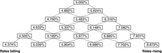
Figure 1 Term Structure Evolution: Binomial Tree
MODELING IN PRACTICE
One popular way of turning theory into practice is to use a tree approach to modeling. The tree can be either binomial or trinomial in its construction. To illustrate the idea, consider first the binomial approach. The tree could be set up to reflect observed or estimated market short rates, and the data provided in Table 1 will help to demonstrate this idea.
The process starts from the first six-month period where the rate is known to be 5.000%. At the end of the six-month period, the following six-month forward rates are treated as being the short rates and are split, allowing interest rates to rise with a probability of 0.5 or fall with a probability of 0.5, but also taking into account the short-rate volatility. For a description of how this is achieved, see Eales (2000). Figure 1 shows how the rates would appear in a binomial tree once the procedure has been performed.
When the rates have been established, they must then be calibrated. The calibration procedure is achieved using the observed market price of a bullet government bond and pricing the bond using the “tree” calculated rates to obtain the appropriate discount factors. Consider a three-year-to-maturity government bond trading at par and offering a coupon of 5.625% paid semiannually as an example. On maturity, the bond will be redeemed for 102.8125, which is made up of the bond's face value, say 100, and one half of the annual coupon, 2.8125.
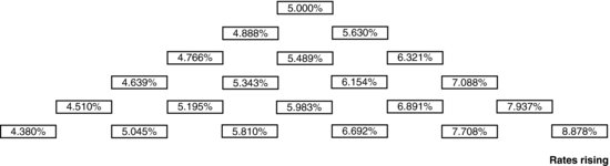
Figure 2 illustrates how, moving back through the tree, the discounting process of the terminal payment taken together with the discounted interim coupons generate a bond price of 100.013. Given that the observed bond price is 100, the rates in the tree will need to be adjusted to ensure that the backward calculated price agrees with the market price of the bond. In this example the adjustment factor is 0.6 basis points, and this will be added to every node in the tree with the exception of the starting value. The resulting rates will then be as displayed in Figure 13.3.
Figure 2 Calibration
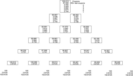
Figure 3 Adjusted Tree to Coincide with Current Market Price
The calibrated tree can now be used to calculate corporate bond spreads as well as bond options. The outlined procedure is close to that advanced by Black, Derman, and Toy in that the process fits observed market rates and short-rate volatility. There is, however, a danger that interest rates could go negative in this procedure.
As an alternative to this binomial approach, Hull and White (1994) have suggested a two-stage methodology that uses a mean-reverting process with the short rate as the source of uncertainty and calculated in a trinomial tree framework.The first stage in the approach ignores the observed market rates and centers the evolution of rates around zero and identifies the point at which the mean-reversion process takes effect. The second stage introduces the observed market rates into the framework established in stage one. The trinomial approach gives the tree a great deal more flexibility over its binomial counterpart, not least in relaxing the assumption that rates can either rise or fall with probability 0.5.
HJM METHODOLOGY
Heath, Jarrow, and Morton (1990a, 1990b, 1992) derived both one-factor and multifactor models for movements of the forward rates of interest. The models were complex enough to match the current observable term structure of forward rate and by equivalence the spot rates. Ritchken and Sankarasubramanian (1995) provide necessary and sufficient conditions for the HJM models with one source of error and two state variables such that the ex post forward premium and the integrated variance factor are sufficient statistics for the construction of the entire term structure at any future point in time.
Under this methodology, the bond dynamics are described by an Ito process:
(29) ![]()
Then
(30) ![]()
The equation for the forward rate can be derived now:
(31) 
The Wiener process W = {W(t)} is symmetric, and therefore we can safely replace W with –W, so
(32) ![]()
Applying the fundamental theorem of calculus for ![]() leads to
leads to
(33) ![]()
It is obvious that ![]() and therefore the volatility of the forward rate determines the drift as well. In other words, all that is needed for the HJM methodology is the volatility of the bond prices. The short rates are easily calculated from the forward rates. Once a model for short rates is determined under the risk-neutral measure Q, the bond prices are calculated from
and therefore the volatility of the forward rate determines the drift as well. In other words, all that is needed for the HJM methodology is the volatility of the bond prices. The short rates are easily calculated from the forward rates. Once a model for short rates is determined under the risk-neutral measure Q, the bond prices are calculated from
(34) ![]()
Using (3) it follows that ![]() where
where
(35) ![]()
The continuous variant of the Ho-Lee model can be obtained for
(36) 
where ![]() , which implies that
, which implies that ![]() so the initial forward curve is
so the initial forward curve is
(37) 
The short rate is given by
(38) ![]()
and the price of the pure discount bond with maturity T is
(39) 
Similarly, the Vasicek model is recovered for
(40) 
and this leads to
(41) ![]()
BOND OPTION PRICING
Formulae for bond options were found by Cox, Ingersoll, and Ross using the CIR model (square root process) for short rates and by Jamshidian (1989), Rabinovitch (1989), and Chaplin (1987) using the Vasicek model for the short-rate process. Rabinovitch advocated the idea that the bond follows a lognormal process (similar to equity prices). Chen (1991) pointed out that this assumption is grossly misleading since the bond price is a contingent claim on the same interest rate, so the bond option pricing model cannot be a two-factor model as proposed by Rabinovitch and it rather collapses onto a one-factor model, in which case the formulas are the same with those proved respectively by Chaplin (1987) and by Jamshidian (1989).
Bonds are traded generally over the counter. Futures contracts on bonds may be more liquid and may remove some of the modeling difficulties generated by the known value at maturity of the bonds. Hedging may be more efficient in this context using the futures contracts on pure discount bonds (provided they are liquid) rather than the bonds themselves. Chen (1992) provides closed-form solutions for futures and European futures options on pure discount bonds, under the Vasicek model.
Hull and White used a two-factor version of the Vasicek model to price discount bond options. Turnbull and Milne (1991) proposed a general equilibrium model outside the HJM framework. They provide analytical solutions for European options on Treasury bills, interest rate forward and futures contracts, and Treasury bonds. In addition, a closed formula is identified for a call option written on an interest rate cap. A two-factor model is also investigated, and closed-form solutions are provided for a European call on a Treasury bill. Chen and Scott (1992) use a two-factor CIR model that is essentially the same as the model analyzed by Longstaff and Schwartz (1992), and derive solutions for bond and interest rate options. The two-factor model is used, with the first factor having a strong mean reversion, explaining the variation in short-term rates, while the second factor has a very slow mean reversion, modeling long-term rates. The model is also used for calculating premiums for caps on floating interest rates and for European options on discount bonds, coupon bonds, coupon bond futures, and Eurodollar futures. These are not closed-form solutions, but they are expressed as multivariate integrals. However, the calculus can be reduced to univariate numerical integrations.
European Options on the Money Fund
In this section we consider the pricing of a European option on the money fund (this is the same as a bank account when the initial value B(0) =1). Thus, the payoff of a European call option with exercise price K is ![]() . The continuous version of the Ho-Lee model is assumed for the short interest rate process. The risk-neutral valuation methodology provides the solution as
. The continuous version of the Ho-Lee model is assumed for the short interest rate process. The risk-neutral valuation methodology provides the solution as
(42) ![]()
where
A proof of this formula is described in Epps (2000) in Section 10.2.2.
Options on Discount Bonds
Discount bond options are not very liquid, but they form an elementary component for pricing other options. For example, a floating rate cap can be decomposed into a portfolio of European puts on discount bonds. Similarly, with the European option contingent to the bank account, we can price European options contingent on discount bonds.
When the short rate process r = {r(t)} follows the continuous time version of the Ho-Lee model given above by (10), the price at time 0 of a European call option with maturity ![]() with exercise price K on a discount bond maturing at T (
with exercise price K on a discount bond maturing at T (![]() ) is
) is
(43) 
where
A proof of this result is provided in Epps (2000). There is a similar put-call parity for European options contingent on a discount bond. If ![]() is the price at t = 0 of a European put option on the discount bond with maturity T, then for
is the price at t = 0 of a European put option on the discount bond with maturity T, then for ![]() ,
,
Put-call parity can be used to derive the price of a European put option:
(44) 
Initially, the first formulas on pricing options on pure discount bonds used the Vasicek model for the term structure of interest rates. Thus, given that r follows (6), the price of a European call option with maturity ![]() with exercise price K on a discount bond maturing at T (
with exercise price K on a discount bond maturing at T (![]() ) is
) is
(45) ![]()
where ![]() , with
, with ![]()
The put price can be obtained from put-call parity as
(46) ![]()
Example: Valuing a Zero-Coupon Bond Call Option with the Vasicek Model
Let's consider this model for pricing a 3-year European call option on a 10-year zero-coupon bond with face value $1 and exercise price K equal to $0.5. As in Jackson and Staunton (2001), we use for the parameters of this model the values estimated by Chan et al. (1992) for U.S. 1-month Treasury bill yield from 1964 to 1989. Thus, ![]() , and
, and ![]() . In addition, the value of the short rate r at time t = 0 is needed, so we take
. In addition, the value of the short rate r at time t = 0 is needed, so we take ![]() . Feeding this information into the above formulas, we get the output in Table 2. Thus, the value of the European call option is
. Feeding this information into the above formulas, we get the output in Table 2. Thus, the value of the European call option is
Table 2 Calculations of Elements for Pricing a European Call Option on a Zero-Coupon Bond When Short Rates Are Following the Vasicek Model
![]()
A more general case is discussed by Shiryaev (1999) for single-factor Gaussian models modeling the short interest rate. These are single-factor affine models where the short rate r is also a Gauss-Markov process. The equation for this short rate process is
(47) ![]()
and we can easily recognize the first Hull-White model. The price of a European call option is also
but where
with
![]()
The price of the European put option is obviously again ![]() .
.
Example: Valuing a Zero-Coupon Bond Call Option with the Hull-White Model
When considering the pricing of a forward pure discount bond earlier in this entry, we used a numerical example. That example can now be expanded to demonstrate how, in practice, European calls and puts can be estimated in a Hull-White framework. Explicitly, the illustration will demonstrate the pricing of a one-year European call option on a four-year-to-maturity discount bond with a strike price set equal to the forward price of the bond (0.8858…).
Breaking down (d+) into its component parts and evaluating each individually yields:
The expression for (d+) reduces to
![]()
The expression for ![]() is
is ![]() .
. ![]() is found to be 0.5255 and
is found to be 0.5255 and ![]() . Substituting these results into the call option formula gives a premium of
. Substituting these results into the call option formula gives a premium of
or 1.73%.
One notable exception from this general class is the CIR model. There is a closed formula for this case, too. Following Clewlow and Strickland (1998), the price at time 0 of a European pure discount bond option is
where
and ![]() is the noncentral chi-squared density with a degrees of freedom and noncentrality parameter b.
is the noncentral chi-squared density with a degrees of freedom and noncentrality parameter b.
Example: Valuing a Zero-Coupon Bond Call Option with the CIR Model
Let's consider the same problem as described in the example using the Vasicek model above and price the 3-year European call option on a 10-year pure discount bond using the CIR model for the short interest rates. Recall that face value is $1 and exercise price K is equal to $0.5. As in the example with the Vasicek model, we consider that ![]() and
and ![]() . The CIR model overcomes the problem of negative interest rates known for the Vasicek model as long as
. The CIR model overcomes the problem of negative interest rates known for the Vasicek model as long as ![]() . This is true, for example, if we take
. This is true, for example, if we take ![]() . Feeding this information into the above formulas is relatively tedious. A spreadsheet application is provided by Jackson and Staunton. After some work, we get that the price of the call is
. Feeding this information into the above formulas is relatively tedious. A spreadsheet application is provided by Jackson and Staunton. After some work, we get that the price of the call is
![]()
Options on Coupon-Paying Bonds
When short rates are modeled with single-factor models, Jamshidian (1989) proved that an option on a coupon bond can be priced by valuing a portfolio of options on discount bonds. This approach does not work in multifactor models as proved by El Karoui and Rochet (1995).
Consider a bond paying a periodic cash payment ρ at times ![]() , and the principal at maturity
, and the principal at maturity ![]() . A coupon bond can be mapped into a portfolio of discount bonds with corresponding maturities (under one source of uncertainty, that is, one factor model). The value of a coupon-bearing bond at time
. A coupon bond can be mapped into a portfolio of discount bonds with corresponding maturities (under one source of uncertainty, that is, one factor model). The value of a coupon-bearing bond at time ![]() is
is
where ![]() .
.
Under the one-factor HJM model corresponding to the Ho-Lee model, a European option on a coupon bond can be valued as a portfolio of options contingent on zero discount bonds with maturities ![]() . Let
. Let ![]() be the maturity of such a European option.
be the maturity of such a European option.
Epps (2000) shows that
(51) ![]()
For any strike price K, there is a value ![]() of
of ![]() such that when replaced in (48) with
such that when replaced in (48) with ![]() , implies
, implies ![]() . Let's denote by
. Let's denote by ![]() the value of
the value of ![]() as calculated from (49) with
as calculated from (49) with ![]() instead of
instead of ![]() . Then
. Then
(52) ![]()
Hence, the value at time 0 of a European call option with maturity ![]() and strike price K on the coupon-bearing bond, under the one-factor HJM model described above, is given by
and strike price K on the coupon-bearing bond, under the one-factor HJM model described above, is given by
(53) 
Example: Valuing a Coupon-Bond Call Option with the Vasicek Model
The above example is reconsidered using the Vasicek model for the short-term interest rates. The bond is no longer a zero-bond but now pays an annual coupon at a 5% rate (ρ = 0.05), all the other characteristics being the same as before. In order to calculate the European call option price on the coupon bond, we need to calculate the interest rate ![]() such that the present value at the maturity of the option of all later cash flows on the bond equals the strike price. This is done by trial and error using (48), and the value we get here is
such that the present value at the maturity of the option of all later cash flows on the bond equals the strike price. This is done by trial and error using (48), and the value we get here is ![]() %. Next, we map the strike price into a series of strike prices via (50) that are then associated with coupon payments considered as zero-coupon bonds and calculate the value of the European call options contingent on those zero-coupon bonds as in the preceding example. The calculations are described in Table 3.
%. Next, we map the strike price into a series of strike prices via (50) that are then associated with coupon payments considered as zero-coupon bonds and calculate the value of the European call options contingent on those zero-coupon bonds as in the preceding example. The calculations are described in Table 3.
Table 3 Calculations Using the Vasicek Model for Separate Zero-Coupon European Call Options (bond prices shown are calculated with the estimated rK)
Because we started with a one-factor model for the short interest rates, we can use the decomposition property emphasized by Jamshidian (1997) and calculate the required coupon-bond European call price as the sum of all the elements in the last column in Table 3, which includes the coupon rate factor ρ. Thus, the value of this option is 0.344.
Example: Valuing a Coupon-Bond Call Option with the CIR Model
We repeat the calculation of the coupon-bond call option when the CIR model is employed for the short rates. The procedure is the same as in the case discussed previously for the Vasicek model. First, we calculate the interest rate ![]() such that the present value at the maturity of the option of all later cash flows on the bond equals the strike price. This value is here
such that the present value at the maturity of the option of all later cash flows on the bond equals the strike price. This value is here ![]() = 25.05%. Next, we map the strike price into a series of strike prices via (50) that are then associated with coupon payments considered as zero-coupon bonds and calculate the value of the European call options contingent to those zero-coupon bonds. The calculations are described in Table 4.
= 25.05%. Next, we map the strike price into a series of strike prices via (50) that are then associated with coupon payments considered as zero-coupon bonds and calculate the value of the European call options contingent to those zero-coupon bonds. The calculations are described in Table 4.
Table 4 Calculations Using the CIR Model for Separate Zero-Coupon European Call Options (bond prices shown are calculated with the estimated rK)
The value of the call option is 0.334, that is, the sum of all zero-coupon bond call option prices in the last column.
Pricing Swaptions
Swaptions options allow the buyer to obtain at a future time one position in a swap contract. It is elementary that an interest rate swap, fixed for floating, can be understood as a portfolio of bonds. Let's consider here that the notional principal is 1. Then the claim on the fixed payments is the same as a bond paying coupons with the rate ρ and no principal. Let τ be the time when the swap is conceived. The claim on the fixed income stream is worth, at time τ, ![]() . The floating income stream is made up of cash returns on holding, over the period
. The floating income stream is made up of cash returns on holding, over the period ![]() a discount bond with maturity Ti, which is worth
a discount bond with maturity Ti, which is worth ![]() . Thus, the value of the whole floating stream at time t = τ is
. Thus, the value of the whole floating stream at time t = τ is
(54) 
Applying the properties of conditional expectations it follows that the above is equal to
(55) 
Imposing the condition that the two streams have equal initial value leads to
![]()
which is equivalent to
![]()
It follows then that the value of the swap at initialization is ![]() Thus, the option to get a long position in the fixed leg of the swap, with a fixed payment rate ρ, is worth at time 0
Thus, the option to get a long position in the fixed leg of the swap, with a fixed payment rate ρ, is worth at time 0
(56) ![]()
It is clear now that this is the same as a European call option on a coupon-bearing bond when the exercise price is equal to 1.
PRACTICAL CONSIDERATIONS
As mentioned in the introduction, the 10-year U.S. Treasury note option traded on the CME is an extremely popular contract offering tight bid/ask spreads and transparent price quotes.
The Eurodollar futures option traded on the CME is the most actively traded short-term interest rate option in the world. If the option contracts are exercised, the buyer and the seller of the option take positions in the Eurodollar futures contract, which is cash-settled, and the final price at delivery is equal to 100 minus the three-month US dollar LIBOR.
Another liquid interest rate derivative market is the OTC in floating rate caps. The majority of caps are contingent on LIBOR (but can be also on a Treasury rate), and discounted payments are made at the beginning of each tenor. The payments can be made either at the beginning or the end of each reset period, and the life of a cap may be only a few years or as long as 10 years. The starting point in pricing these European options is a model for future changes in US dollar LIBOR.
Hull and White (1990) showed that the cap can be priced as a portfolio of European puts on discount bonds.
KEY POINTS
- One-factor short-rate models for interest rate derivatives are easy to work with since the majority of them lead to closed-form solutions for options pricing. However, some of them allow for negative interest rates, which may not be acceptable in a real trading environment.
- Two-factor models for interest rates provide improved calibration at the expense of computational simplicity.
- The two-factor Hull and White model, falling under the general Heath-Jarrow-Morton framework, is complex enough to calibrate market data easily while retaining computational simplicity through closed-form solutions for a wide range of interest rate derivatives.
- The need for improved calibration of forward curves led to the development of a different class of models called LIBOR models.
- The calibration of caps and floors, and also swaptions, is indicative of the success of an interest rate model.
REFERENCES
Black, F., Derman, E., and Toy, W. (1990). A one-factor model of interest rate and its application to Treasury bond options. Financial Analysts Journal 46: 33–39.
Black, F., and Karasinski, P. (1991). Bond and option pricing when short rates are lognormal. Financial Analysts Journal 47: 52–59.
Brennan, M. J., and Schwartz, E. (1979). A continuous time approach to the pricing of bonds. Journal of Banking and Finance 3: 133–155.
Brace, A., Gatarek, D., and Musiela, M. (1997). The market model of interest rate dynamics. Mathematical Finance 7: 127–155.
Brennan, M. J., and Schwartz, E. (1982). An equilibrium model of bond prices and a test of market efficiency. Journal of Financial and Quantitative Analysis 17: 301–329.
Brigo, D., and Mercurio, F. (2007). Interest Rate Models: Theory and Practice, 2nd edition. Berlin: Springer.
Campbell, J. (1986). A defense of traditional hypotheses about the term structure of interest rates. Journal of Finance 41, 1: 183–194.
Chen, L. (1995). A three-factor model of the term structure of interest rates. Preprint, Federal Reserve Board, Washington, July.
Chen, R. R. (1991). Pricing stock and bond options when the default-free rate is stochastic: A comment. Journal of Financial and Quantitative Analysis 26, 3: 433–434.
Chen, R. R. (1992). Exact solutions for futures and European futures options on pure discount bonds. Journal of Financial and Quantitative Analysis 27, 1: 97–107.
Chen, R. R., and Scott, L. (1992). Pricing interest rate options in a two-factor Cox-Ingersoll-Ross model of the term structure. Review of Financial Studies 5, 4: 613–636.
Chaplin, G. (1987). A formula for bond option values under an Ornstein-Uhlenbeck model for the spot. Actuarial Science working paper No. 87–16, University of Waterloo.
Clewlow, L., and Strickland, C. (1998). Implementing Derivatives Models. Chichester, UK: John Wiley & Sons.
Constantinides, G. M. (1992). A theory of the nominal term structure of interest rates. Review of Financial Studies 5, 4: 531–552.
Courtadon, G. (1982). The pricing of default-free bonds. Journal of Financial and Quantitative Analysis 17: 75–100.
Cox, J. C., Ingersoll, J. E., and Ross, S. A. (1980). An analysis of variable rate loan contracts. Journal of Finance 35: 389–403.
Cox, J. C., Ingersoll, J. E., and Ross, S. A. (1985). A theory of the term structure of interest rates. Econometrica 53, 2: 385–407.
Dothan, M. U. (1978). On the term structure of interest rates. Journal of Financial Economics 6: 9–69.
Eales, B. A. (2000). Financial Engineering. New York: Palgrave Macmillan.
Epps, T. W. (2000). Pricing Derivative Securities. Singapore: World Scientific.
El Karoui, N., and Rochet, J. C. (1995). A price formula for options on coupon bonds. SEEDS Discussion Series, Instituto de Economica Publica, Spain.
Flesaker, B., and Hughston, L. P. (1996). Positive interest. Risk 9, 1: 115–124.
Fong, H. G., and Vasicek, O. A. (1992). Interest rate volatility and a stochastic factor. Working paper, Gifford Fong Associates.
Heath, D., Jarrow, R., and Morton, A. (1990a). Bond pricing and the term structure of interest rates: A discrete time approximation. Journal of Financial and Quantitative Analysis 25: 419–440.
Heath, D., Jarrow, R., and Morton, A. (1990b). Contingent claim valuation with a random evolution of interest rates. Review of Futures Markets 9: 54–76.
Heath, D., Jarrow, R., and Morton, A. (1992). Bond pricing and the term structure of interest rates. Econometrica 60, 1: 77–105.
Ho, T., and Lee, S. (1986). Term structure movements and pricing interest rates contingent claims. Journal of Finance 41: 1011–1029.
Hull, J. C. (2003). Options, Futures, and Other Derivatives. Upper Saddle River, NJ: Prentice Hall.
Hull, J. C., and White, A. (1990). Pricing interest rate derivative securities. Review of Financial Studies 3, 5: 573–592.
Hull, J. C., and White, A. (1994). Numerical procedures for implementing term structure models I: Single-factor models. Journal of Derivatives 2, 1: 7–16.
Hull, J. C., and White, A. (1996). Using Hull-White interest rate trees. Journal of Derivatives, Spring: 26–36.
Jamshidian, F. (1989). An exact bond option formula. Journal of Finance 44, 1: 205–209.
Jamshidian, F. (1997). LIBOR and swap market models and measures. Finance and Stochastics 1: 293–330.
Longstaff, F. A., and Schwartz, E. S. (1992a). Interest rate volatility and the term structure: A two-factor general equilibrium model. Journal of Finance 47: 1259–1282.
Longstaff, F. A., and Schwartz, E. S. (1992b). A two-factor interest rate model and contingent claim valuation. Journal of Fixed Income 3: 16–23.
Mercurio, F., and Moraleda, J. M. (2000). An analytically tractable interest rate model with humped volatility. European Journal of Operational Research 120: 205–214.
Merton, R. C. (1973). Theory of rational option pricing. Bell Journal of Economics and Management Science 4, Spring: 141–183.
Musiela, M., and Rutkowski, M. (1997). Martingale Methods in Financial Modelling. Berlin: Springer.
Rabinovitch, R. (1989). Pricing stock and bond options when the default-free rate is stochastic: A comment. Journal of Financial and Quantitative Analysis 24, 4: 447–457.
Rebonato, R. (1998) Interest-Rate Option Models, 2nd Edition. Chichester, UK: John Wiley & Sons.
Rendleman, R., and Bartter, B. (1980). The pricing of options on debt securities. Journal of Financial and Quantitative Analysis 15: 11–24.
Rogers, L.C.G. (1997). The potential approach to the term structure of interest rates and foreign exchange rates. Mathematical Finance 7: 157–176.
Ritchken, P., and Sankarasubramanian, L. (1995). Volatility structures of forward rates and the dynamics of the term structure. Mathematical Finance 5: 55–72.
Rutkowski, M. (1997). Models of forward LIBOR and swap rates. Preprint, University of New South Wales.
Sandmann, K., and Sondermann, D. (1993). A term structure model and the pricing of interest rate derivatives. Review of Futures Markets 12, 2: 391–423.
Schmidt, W. M. (1997). On a general class of one-factor models for the term structure of interest rates. Finance and Stochastics 1: 3–24.
Strickland, C. R. (1992). The delivery option in bond futures contracts: An empirical analysis of the LIFFE long gilt futures contract. Review of Futures Markets 11: 84–102.
Shiryaev, A. N. (1999). Essentials of Stochastic Finance: Facts, Models, Theory. Singapore: World Scientific.
Turnbull, S. M., and Milne, F. (1991). A simple approach to interest-rate option pricing. Review of Financial Studies. 4, 1: 87–120.
Vasicek, O. (1977). An equilibrium characterization of the term structure. Journal of Financial Economics 5: 177–188.