Modeling Asset Price Dynamics

DESSISLAVA A. PACHAMANOVA, PhD

Associate Professor of Operations Research, Babson College

FRANK J. FABOZZI, PhD, CFA, CPA

Professor of Finance, EDHEC Business School

Many classical asset pricing models, such as the capital asset pricing theory and the arbitrage pricing theory, take a myopic view of investing: They consider events that happen one time period ahead, where the length of the time period is determined by the investor. This entry presents apparatus that can handle asset dynamics and volatility over time. The dynamics of price processes in discrete time increments are typically described by two kinds of models: trees (such as binomial trees) and random walks. When the time increment used to model the asset price dynamics becomes infinitely small, we talk about stochastic processes in continuous time.

In this entry, we introduce the fundamentals of binomial tree and random walk models, providing examples for how they can be used in practice. We briefly discuss the special notation and terminology associated with stochastic processes at the end of the entry; however, our focus is on interpretation and simulation of processes in discrete time. The roots for the techniques we describe are in physics and the other natural sciences. They were first applied in finance at the beginning of the 20th century and have represented the foundations of asset pricing ever since.

FINANCIAL TIME SERIES

Let us first introduce some definitions and notation. A financial time series is a sequence of observations of the values of a financial variable, such as an asset price (index level) or asset (index) returns, over time. Figure 1 shows an example of a time series, consisting of weekly observations of the S&P 500 price level over a period of five years (August 19, 2005 to August 19, 2009).

When we describe a time series, we talk about its drift and volatility. The term “drift” is used to indicate the direction of any observable trend in the time series. In the example shown in Figure 1, it appears that the S&P 500 time series has a positive drift up from August 2005 until about the middle of 2007, as the level of prices appears to have been generally increasing over that time period. From the middle of 2007 until the beginning of 2009, there is a negative drift. The volatility is smaller (the time series is less “squiggly”) from August 2005 until about the middle of 2007, but increases dramatically between the middle of 2007 and the beginning of 2009.

Figure 1 S&P 500 Index Level between August 19, 2005 and August 19, 2009

We are usually interested also in whether the volatility increases when the price level increases, decreases when the price level decreases, or remains constant independently of the current price level. In this example, the volatility is lower when the price level is increasing, and is higher when the price level is decreasing.

Finally, we talk about the continuity of the time series—is the time series smooth, or are there jumps whose magnitude appears to be large relative to the price movements the rest of the time? From August 2005 until about the middle of 2007, the time series is quite smooth. However, some dramatic drops in price levels can be observed between the middle of 2007 and the beginning of 2009—notably in the fall of 2008.

For the remainder of this entry, we will use the following notation:

• St: value of underlying variable (price, interest rate, index level, etc.) at time t.
• St+1: value of underlying variable (price, interest rate, etc.) at time t +1.
• ωt: a random error term observed at time t. (For the applications in this entry, it will follow a normal distribution with mean equal to 0 and standard deviation equal to σ.)
• ɛt: a realization of a normal random variable with mean equal to 0 and standard deviation equal to 1 at time t.

BINOMIAL TREES

Binomial trees (also called binomial lattices) provide a natural way to model the dynamics of a random process over time. The initial value of the security S0 (at time 0) is known. The length of a time period, Δt, is specified before the tree is built. (The symbol Δ is often used to denote difference. The notation Δt therefore means time difference, i.e., length of one time period.)

The binomial tree model assumes that at the next time period, only two values are possible for the price, that is, the price may go up with probability p or down with probability (1 – p) . Usually, these values are represented as multiples of the price at the beginning of the period. The factor u is used for an up movement, and d is used for a down movement. For example, the two prices at the end of the first time period are u·S0 and d·S0. If the tree is recombining, there will be three possible prices at the end of the second time period: u2·S0, u·d·S0, and d2·S0. Proceeding in a similar manner, we can build the tree in Figure 2.

Figure 2 Example of a Binomial Tree

Figure 3 Binomial Distribution

Note: Probability of success (p) assumed to be 0.3. Number of trials (A) n = 3; (B) n = 20; (C) n = 100.

The binomial tree model may appear simple, because, given a current price, it only allows for two possibilities for the price at each time period. However, if the length of the time period is small, it is possible to represent a wide range of values for the price after only a few steps. To see this, notice that each step in the tree can be thought of as a Bernoulli trial—it is a “success” with probability p and a “failure” with probability (1 – p). (One can think of the Bernoulli random variable as the numerical coding of the outcome of a coin toss, where one outcome is considered a “success” and one outcome is considered a “failure.” The Bernoulli random variable takes the value 1 (“success”) with probability p and the value of 0 (“failure”) with probability 1 – p. Note that the definition of success and failure here is arbitrary, because an increase in price is not always desirable, but we define them in this way for the example’s sake.)

After n steps, each particular value for the price will be reached by realizing k successes and (n – k) failures, where k is a number between 0 and n. The probability of reaching each value for the price after n steps will be

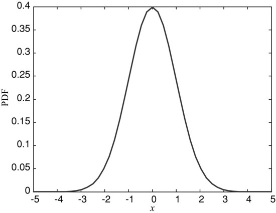
For large values of n, the shape of the binomial distribution becomes more and more symmetric and looks like a continuum. (See Figure 3(A)–(C).) In fact, the binomial distribution approximates a normal distribution with specific mean and standard deviation related to the probability of success and the number of trials. (The normal distribution is a continuous probability distribution. It is represented by a bell-shaped curve, and the shape of the curve is entirely described by the distribution mean and variance. Figure 4 shows a graph of the standard normal distribution, which has a mean of zero and a standard deviation of 1.) One can therefore represent a large range of values for the price as long as the number of time periods used in the binomial tree is large. Practitioners often use also trinomial trees, that is, trees with three branches emanating from each node, in order to obtain a better representation of the range of possible prices in the future.

Figure 4 Standard Normal Distribution

ARITHMETIC RANDOM WALKS

Instead of assuming that at each step the asset price can only move up or down by a certain multiple with a given probability, we could assume that the price moves by an amount that follows a normal distribution with mean μ and standard deviation σ. In other words, the price for each period is determined from the price of the previous period by the equation

where is a normal random variable with mean 0 and standard deviation σ. We will also assume that the random variable describing the change in the price in one time period is independent of the random variables describing the change in the price in any other time period. (This is known as the Markov property. It implies that past prices are irrelevant for forecasting the future, and only the current value of the price is relevant for predicting the price in the next time period.) A sequence of independent and identically distributed (IID) random variables , … , , … with zero mean and finite variance σ2 is sometimes referred to as white noise.

The movement of the price expressed through the equation above is called an arithmetic random walk with drift. The drift term, μ, represents the average change in price over a single time period. Note that for every time period t, we can write the equation for the arithmetic random walk as

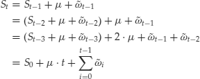
Therefore, an arithmetic random walk can be thought of as a sum of two terms: a deterministic straight line St = S0 + μ·t and a sum of all past noise terms. (See Figure 5.)

Figure 5 Five Paths of an Arithmetic Random Walk Assuming μ = –0.1697 and σ = 3.1166

Simulation

The equation for the arithmetic random walk can be expressed also as

where is a standard normal random variable. To show this, we need to mention that every normal distribution can be expressed in terms of the standard normal distribution, and the latter has mean of 0 and standard deviation of 1. Namely, if is a standard normal variable with mean 0 and standard deviation 1, and is a normal random variable with mean μ and standard deviation σ, we have

This is a property unique to the normal distribution—no other family of probability distributions can be transformed in the same way. In the context of the equation for the arithmetic random walk, we have a normal random variable with mean 0 and standard deviation σ. It can be expressed through a standard normal variable as .

The equation for St+1 above makes it easy to generate paths for the arithmetic random walk by simulation. All we need is a way of generating the standard normal random variables . We start with an initial price S0, which is known. We also know the values of the drift μ and the volatility σ over one period. To generate the price at the next time period, S1, we add μ to S0, simulate a normal random variable from a standard normal distribution, multiply it by σ, and add it to S0 + μ. At the next step (time period 2), we use the price at time period 1 we already generated, S1, add to it μ, simulate a new random variable from a standard normal distribution, multiply it by σ, and add it to S1 + μ. We proceed in the same way until we generate the desired number of steps of the random walk. For example, given a current price S, in Excel the price for the next time period can be generated with the formula

Parameter Estimation

In order to simulate paths of the arithmetic random walk, we need estimates of the parameters (μ and σ). We need to assume that these parameters remain constant over the time period of estimation. Note that the equation for the arithmetic random walk can be written as

Given a historical series of T prices for an asset, we can therefore do the following to estimate μ and σ:

An important point to keep in mind is the units in which the parameters are estimated. If we are given time series in monthly increments, then the estimates of μ and σ we will obtain through steps 1–3 will be for monthly drift and monthly volatility. If we then need to simulate future paths for monthly observations, we can use the same μ and σ. However, if, for example, we need to simulate weekly observations, we will need to adjust μ and σ to account for the difference in the length of the time period. In general, the parameters should be stated as annual estimates. The annual estimates can then be adjusted for daily, weekly, monthly, and so on increments.

For example, suppose that we have estimated the weekly drift and the weekly volatility. To convert the weekly drift to an annual drift, we multiply the number we found for the weekly drift by 52, the number of weeks in a year. To convert the weekly volatility to annual volatility, we multiply the number we found for the weekly volatility by the square root of the number of weeks in a year, that is, by . Conversely, if we are given annualized values for the drift and the volatility, we can obtain weekly values by dividing the annual drift and the volatility by 52 and , respectively.

Arithmetic Random Walks: Some Additional Facts

If we use the arithmetic random walk model, any price in the future, St, can be expressed through the initial (known) price S0 as

The random variable corresponding to the sum of t independent normal random variables , … , is a normal random variable with mean equal to the sum of the means and standard deviation equal to the square root of the sum of variances. Since , … , are independent standard normal variables, their sum is a normal variable with mean 0 and standard deviation equal to

Therefore, we can have a closed-form expression for computing the asset price at time t given the asset price at time 0:

where is a standard normal random variable.

Based on the discussion so far in this section, we can state the following observations about the arithmetic random walk:

• The arithmetic random walk has a constant drift μ and volatility σ, that is, at every time period, the change in price is normally distributed, on average equal to μ, with a standard deviation of σ.
• The overall noise in a random walk never decays. The price change over t time periods is distributed as a normal distribution with mean equal to μ·t and standard deviation equal to . That is why in industry one often encounters the phrase “The uncertainty grows with the square root of time.”
• Prices that follow an arithmetic random walk meander around a straight line St = S0 + μ·t. They may depart from the line, and then cross it again.
• Because the distribution of future prices is normal, we can theoretically find the probability that the future price at any time will be within a given range.
• Because the distribution of future prices is normal, future prices can theoretically take infinitely large or infinitely small values. Thus, they can be negative, which is an undesirable consequence of using the model.

Asset prices, of course, cannot be negative. In practice, the probability of the price becoming negative can be made quite small as long as the drift and the volatility parameters are selected carefully. However, the possibility of generating negative prices with the arithmetic random walk model is real.

Another problem with the assumptions underlying the arithmetic random walk is that the change in the asset price is drawn from the same random probability distribution, independently of the current level of the prices. A more natural model is to assume that the parameters of the random probability distribution for the change in the asset price vary depending on the current price level. For example, a $1 change in a stock price is more likely when the stock price is $100 than when it is $4. Empirical studies confirm that over time, asset prices tend to grow, and so do fluctuations. Only returns appear to remain stationary, that is, to follow the same probability distribution over time. A more realistic model for asset prices may therefore be that returns are an IID sequence. We describe such a model in the next section.

GEOMETRIC RANDOM WALKS

Consider the following model:

where , … , is a sequence of independent normal variables, and rt, the return, is computed as

Returns are therefore normally distributed, and the return over each interval of length 1 has mean μ and standard deviation σ. How can we express future prices if returns are determined by the equations above?

Suppose we know the price at time t, St. The price at time t+1 can be written as

This last equation is very similar to the equation for the arithmetic random walk, except that the price from the previous time period appears as a factor in all of the terms.

The equation for the geometric random walk makes it clear how paths for the geometric random walk can be generated. As in the case of the arithmetic random walk, all we need is a way of generating the normal random variables . We start with an initial price S0, which is known. We also know the values of the drift μ and the volatility σ over one period. To generate the price at the next time period, S1, we add μ·S0 to S0, simulate a normal random variable from a standard normal distribution, multiply it by σ and S0, and add it to S0 + μ·S0. At the next step (time period 2), we use the price at time period 1 we already generated, S1, add to it μ·S1, simulate a new random variable from a standard normal distribution, multiply it by σ and S1, and add it to S1 + μ·S1. We proceed in the same way until we generate the desired number of steps of the geometric random walk. For example, given a current price S, in Excel the price for the next time period can be generated with the formula

Using similar logic to the derivation of the price equation earlier, we can express the price at any time t in terms of the known initial price S0. Note that we can write the price at time t as

Therefore,

In the case of the arithmetic random walk, we determined that the price at any time period follows a normal distribution. This was because if we know the starting price S0, the price at any time period could be obtained by adding a sum of independent normal random variables to a constant term and S0. The sum of independent normal random variables is a normal random variable itself. In the equation for the geometric random walk, each of the terms is a normal random variable as well. (It is the sum of a normal random variable and a constant.) However, they are multiplied together. The product of normal random variables is not a normal random variable, which means that we cannot have a nice closed-form expression for computing the price St based on S0.

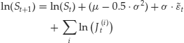
To avoid this problem, let us consider the natural logarithm of prices. (The natural logarithm is the function ln so that eln(x) = x, where e is the number 2.7182 … .) Unless otherwise specified, we will use “logarithm” to refer to the natural logarithm, that is, the logarithm of base e.

If we take logarithms of both sides of the equation for St, we get

Log returns are in fact differences of log prices. To see this, note that

Now assume that log returns (not returns) are independent and follow a normal distribution with mean μ and standard deviation σ:

As a sum of independent normal variables, the expression

is also normally distributed. This means that ln(St) (rather than St) is normally distributed, that is, St is a lognormal random variable. Similarly to the case of an arithmetic random walk, we can compute a closed-form expression for the price St given S0:

or, equivalently,

where is a standard normal variable.

Notice that the only inconsistency with the formula for the arithmetic random walk is the presence of the extra term

in the drift term

Why is there an adjustment of one half of the variance in the expected drift? In general, if is a normal random variable with mean μ and variance σ2, then the random variable, which is an exponential of the normal random variable , , has mean

At first, this seems unintuitive—why is the expected value of not

The expected value of a linear function of a random variable is a linear function of the expected value of the random variable. For example, if a is a constant, then

However, determining the expected value of a nonlinear function of a random variable (in particular, the exponential function, which is the function we are using here) is not as trivial. For example, there is a well-known relationship, the Jensen inequality, which states that the expected value of a convex function of a random variable is less than the value of the function at the expected value of the random variable.

Figure 6 Example of a Lognormal Distribution with Mean of 1 and Standard Deviation of 0.8

In our example, is a lognormal random variable, so its probability distribution has the shape shown in Figure 6. The random variable cannot take values less than 0. Since its variance is related to the variance of the normal random variable , as the variance σ2 of increases, the distribution of will spread out in the upward direction. This means that the mean of the lognormal variable will increase not only as the mean of the normal variable , μ, increases, but also as ’s variance, σ2, increases. In the context of the geometric random walk, represents the normally distributed log returns, and is in fact the factor by which the asset price from the previous period is multiplied in order to generate the asset price in the next time period. In order to make sure that the geometric random process grows exponentially at average rate μ, we need to subtract a term (that term turns out to be σ2/2), which will correct the bias.

Specifically, suppose that we know the price at time t, St. We have

that is,

Note that we are explicitly assuming a multiplicative model for asset prices here—the price in the next time period is obtained by multiplying the price from the previous time period by a random factor. In the case of an arithmetic random walk, we had an additive model—a random shock was added to the asset price from the previous time period.

If the log return ln() is normally distributed with mean μ and standard deviation σ, then the expected value of

is

and hence

In order to make sure that the geometric random walk process grows exponentially at an average rate μ (rather than ), we need to subtract the term 0.5·σ2 when we generate the future price from this process. This argument can be extended to determining prices for more than one time period ahead.

We will understand better why this formula holds when we review stochastic processes at the end of this entry.

Simulation

It is easy to see how future prices can be generated based on the initial price S0. First, we compute the term in the power of e: We simulate a value for a standard normal random variable, multiply it by the standard deviation and the square root of the number of time periods between the initial point and the point we are trying to compute, and subtract the product from the drift term adjusted for the volatility and the number of time periods. We then raise e to the exponent we just computed and multiply the resulting value by the value of the initial price. For example, given a current price S, in Excel we use the formula

One might wonder whether this approach for simulating realizations of an asset price following a geometric random walk is equivalent to the simulation approach mentioned earlier when we introduced geometric random walks, which is based on the discrete version of the equation for a random walk. The two approaches are different (for example, the approach based on the discrete version of the equation for the geometric random walk does not produce the expected lognormal price distribution), but it can be shown that the differences in the two simulation approaches tend to cancel over many steps.

Parameter Estimation

In order to simulate paths of the geometric random walk, we need to have estimates of the parameters (μ and σ). The implicit assumption here, of course, is that these parameters remain constant over the time period of estimation. (We will discuss how to incorporate considerations for changes in volatility later in this entry.) Note that the equation for the geometric random walk can be written as

Equivalently,

Given a historical series of T prices of an asset, we can therefore do the following to estimate μ and σ:

If we are given data on the returns rt of an asset rather than the prices of the asset, we can compute ln(1 + rt), and use it to replace ln(St+1/St) in steps 1–3 above. This is because

Geometric Random Walk: Some Additional Facts

To summarize, the geometric random walk has several important characteristics:

• It is a multiplicative model, that is, the price at the next time period is a multiple of a random term and the price from the previous time period.
• It has a constant drift μ and volatility σ. At every time period, the percentage change in price is normally distributed, on average equal to μ, with a standard deviation of σ.
• The overall noise in a geometric random walk never decays. The percentage price change over t time periods is distributed as a normal distribution with mean equal to μ·t and standard deviation equal to .
• The exact distribution of the future price knowing the initial price can be found. The price at time t is lognormally distributed with specific probability distribution parameters.
• Prices that follow a geometric random walk in continuous time never become negative.

The geometric random walk model is not perfect. However, its computational simplicity makes the geometric random walk and its variations the most widely used processes for modeling asset prices. The geometric random walk defined with log returns never becomes negative, because future prices are always a multiple of the initial stock price and a positive term. (See Figure 7.) In addition, observed historical stock prices can actually be quite close to lognormal.

Figure 7 Five Paths of a Geometric Random Walk with μ = –0.0014 and σ = 0.0411

Note: Although the drift is slightly negative, it is still possible to generate paths that generally increase over time.

It is important to note that, actually, the assumption that log returns are normal is not required to justify the lognormal model for prices. If the distribution of log returns is non-normal, but the log returns are IID with finite variance, the sum of the log returns is asymptotically normal. (This is based on a version of the central limit theorem.) Stated differently, the log return process is approximately normal if we consider changes over sufficiently long intervals of time.

Price processes, however, are not always geometric random walks, even asymptotically. A very important assumption for the geometric random walk is that price increments are independently distributed; if the time series exhibits autocorrelation, the geometric random walk is not a good representation. We will see some models that incorporate considerations for autocorrelation and other factors later in this entry.

MEAN REVERSION

The geometric random walk provides the foundation for modeling the dynamics for asset prices of many different securities, including stock prices. However, in some cases it is not justified to assume that asset prices evolve with a particular drift, or can deviate arbitrarily far from some kind of a representative value. Interest rates, exchange rates, and the prices of some commodities are examples for which the geometric random walk does not provide a good representation over the long term. For instance, if the price of copper becomes high, copper mines would increase production in order to maximize profits. This would increase the supply of copper in the market, therefore decreasing the price of copper back to some equilibrium level. Consumer demand plays a role as well—if the price of copper becomes too high, consumers may look for substitutes, which would reduce the price of copper back to its equilibrium level.

Figure 8 illustrates the behavior of the one-year Treasury bill yield from the beginning of January 1962 through the end of July 2009. It can be observed that, even though the variability of Treasury bill rates has changed over time, there is some kind of a long-term average level of interest rates to which they return after deviating up or down. This behavior is known as mean reversion.

Figure 8 Weekly Data for One-Year Treasury Bill Rates: January 5, 1962–July 31, 2009

The simplest mean reversion (MR) model is similar to an arithmetic random walk, but the means of the increments change depending on the current price level. The price dynamics are represented by the equation

where is a standard normal random variable. The parameter κ is a nonnegative number that represents the speed of adjustment of the mean-reverting process—the larger its magnitude, the faster the process returns to its long-term mean. The parameter μ is the long-term mean of the process. When the current price St is lower than the long-term mean μ, the term (μ – St) is positive. Hence, on average there will be an upward adjustment to obtain the value of the price in the next time period, St+1. (We add a positive number, κ·(μ – St), to the current price St.) By contrast, if the current price St is higher than the long-term mean μ, the term (μ – St) is negative. Hence, on average there will be a downward adjustment to obtain the value of the price in the next time period, St+1. (We add a negative number, κ·(μ – St), to the current price St.) Thus, the mean-reverting process will behave in the way we desire—if the price becomes lower or higher than the long-term mean, it will be drawn back to the long-term mean.

In the case of the arithmetic and the geometric random walks, the cumulative volatility of the process increases over time. By contrast, in the case of mean reversion, as the number of steps increases, the variance peaks at

In continuous time, this basic mean-reversion process is called the Ornstein-Uhlenbeck process. (See the last section of this entry.) It is widely used when modeling interest rates and exchange rates in the context of computing bond prices and prices of more complex fixed-income securities. When used in the context of modeling interest rates, this simple mean-reversion process is also referred to as the Vasicek model (see Vasicek, 1977).

The mean-reversion process suffers from some of the disadvantages of the arithmetic random walk—for example, it can technically become negative. However, if the long-run mean is positive, and the speed of mean reversion is large relative to the volatility, the price will be pulled back to the mean quickly when it becomes negative. Figure 9 contains an example of five paths generated from a mean-reverting process.

Figure 9 Five Paths with 50 Steps Each of a Mean-Reverting Process with μ = 1.4404, κ = 0.0347, and σ = 0.0248

Simulation

The formula for the mean-reverting process makes it clear how paths for the mean-reverting random walk can be generated. As in the case of the arithmetic and the geometric random walks, all we need is a way of simulating the standard normal random variables . We start with an initial price S0, which is known. We know the values of the drift μ, the speed of adjustment κ, and the volatility σ over one period. To generate the price at the next time period, S1, we add κ·(μ – S0) to S0, simulate a normal random variable from a standard normal distribution, multiply it by σ, and add it to S0 + κ·(μ – S0). At the next step (time period 2), we use the price at time period 1 we already generated, S1, add to it κ·(μ – S1), simulate a new random variable from a standard normal distribution, multiply it by σ, and add it to S1 + κ·(μ – S1). We proceed in the same way until we generate the desired number of steps of the random walk. For example, given a current price S, in Excel the price for the next time period can be generated with the formula

Parameter Estimation

In order to simulate paths of the mean-reverting random walk, we need estimates of the parameters (κ, μ, and σ). Again, we assume that these parameters remain constant over the time period of estimation. The equation for the mean-reverting process can be written as

or, equivalently,

This equation has the characteristics of a linear regression model, with the absolute price change (St+1 – St) as the response variable and St as the explanatory variable. Given a historical series of T prices for an asset, we can therefore do the following to estimate κ, μ, and σ:

Geometric Mean Reversion

A more advanced mean-reversion model that bears some similarity to the geometric random walk is the geometric mean reversion (GMR) model

(Note that this is a special case of the mean reversion model St+1 = St + κ·(μ – St)·St + σ··, where γ is a parameter selected in advance. The most commonly used models have γ = 1 or γ = 1/2.) The intuition behind this model is similar to the intuition behind the discrete version of the geometric random walk—the variability of the process changes with the current level of the price. However, the GMR model allows for incorporating mean reversion. Even though it is difficult to estimate the future price analytically from this model, it is easy to simulate. For example, given a current price S, in Excel the price for the next time period can be generated with the formula

Figure 10 contains an example of five paths generated from a geometric mean reversion model.

Figure 10 Five Paths with 50 Steps Each of a Geometric Mean Reversion Process with μ = 1.4464, κ = 0.0253, and σ = 0.0177

To estimate the parameters κ, μ, and σ to use in the simulation, we can use a series of T historical observations for the price of an asset. Assume that the parameters of the geometric mean reversion remain constant during the time period of estimation.

Note that the equation for the geometric mean-reverting random walk can be written as

or, equivalently, as

Again, this equation bears characteristics of a linear regression model, with the percentage price change (St+1 – St)/St as the response variable and St as the explanatory variable. Given a historical series of T prices of an asset, we can therefore do the following to estimate κ, μ, and σ:

ADVANCED RANDOM WALK MODELS

The models we described so far provide building blocks for representing the asset price dynamics. However, observed real-world asset price dynamics has features that cannot be incorporated in these basic models. For example, asset prices exhibit correlation—both with each other and with themselves over time. Their volatility typically cannot be assumed to be constant. This section reviews several techniques for making asset price models more realistic depending on observed price behavior.

Correlated Random Walks

So far, we have discussed models for asset prices that assume that the dynamic processes for the prices of different assets evolve independently of each other. This is an unrealistic assumption—it is expected that market conditions and other factors will have an impact on the prices of groups of assets simultaneously. For example, it is likely that stock prices for companies in the oil industry will generally move together, as will stock prices for companies in the telecommunications industry.

The argument that asset prices are codependent has theoretical and empirical foundations as well. If asset prices were independent random walks, then large portfolios would be fully diversified, have no variability, and therefore be completely deterministic. Empirically, this is not the case. Even large aggregates of stock prices, such as the S&P 500, exhibit random behavior.

If we make the assumption that log returns are jointly normally distributed, then their dependencies can be represented through the covariance matrix (equivalently, through the correlation matrix). It is worth noting that in general, covariance and correlation are not equivalent with dependence of random variables. Covariance and correlation measure only the strength of linear dependence between two random variables. However, in the case of a multivariate normal distribution, covariance and correlation are sufficient to represent dependence.

Let us give an example of how one can model two correlated stock prices assumed to follow geometric random walks. Suppose we are given two historical series of T observations each of observed asset prices for Stock 1 and Stock 2. We follow the steps described in the previous sections of this entry to estimate the drifts and the volatilities of the two processes. To estimate the correlation structure, we find the correlation between

where the indices (1) and (2) correspond to Stock 1 and Stock 2, respectively. For example, in Excel the correlation between two data series stored in Array1 and Array2 can be computed with the function CORREL(Array1, Array2). This correlation can then be incorporated in the simulation. (Excel cannot simulate correlated normal random variables. A number of Excel add-ins for simulation are available, however, and they have the capability to do so. Such add-ins include @RISK (sold by Palisade Corporation, http://www.palisade.com), Crystal Ball (sold by Oracle, http://www.oracle.com), and Risk Solver (from Frontline Systems, the developers of the original Excel Solver, http://www.solver.com).) Basically, at every step, we generate correlated normal random variables, and , with means of zero and with a given covariance structure. Those realizations of the correlated normal random variables are then used to compute the next period’s Stock 1 price and the next period’s Stock 2 price.

When we consider many different assets, the covariance matrix becomes very large and cannot be estimated accurately. Factor models can be used to reduce the dimension of the covariance structure. Multivariate random walks are in fact dynamic factor models for asset prices. A multifactor model for the return of asset i can be written in the following general form:

where the K factors f(k) follow random walks, are the factor loadings, and are normal random variables with zero means.

It is important to note that the covariance matrix cannot capture correlations at lagged times (i.e., correlations of dynamic nature). Furthermore, the assumptions that log returns behave as multivariate normal variables is not always applicable—some assets exhibit dependency of a nonlinear kind, which cannot be captured by the covariance or correlation matrix. Alternative tools for modeling covariability include copula functions and transfer entropies. (See, for example, Chapter 17 and Appendix B in Fabozzi, Focardi, and Kolm, 2006.)

Incorporating Jumps

Many of the dynamic asset price processes used in industry assume continuous sample paths, as was the case with the arithmetic, geometric, and the different mean-reverting random walks we considered earlier in this entry. However, there is empirical evidence that the prices of many securities incorporate jumps. The prices of some commodities, such as electricity and oil, are notorious for exhibiting “spikes.” The logarithm of a price process with jumps is not normally distributed, but is instead characterized by a high peak and heavy tails, which are more typical of market data than the normal distribution. Thus, more advanced models are needed to incorporate realistic price behavior.

A classical way to include jumps in models for asset price dynamics is to add a Poisson process to the process (geometric random walk or mean reversion) used to model the asset price. A Poisson process is a discrete process in which arrivals occur at random discrete points in time, and the times between arrivals follow an exponential distribution with average time between arrivals equal to 1/λ. This means that the number of arrivals in a specific time interval follows a Poisson distribution with mean rate of arrival λ. The “jump” Poisson process is assumed to be independent of the underlying “smooth” random walk.

The Poisson process is typically used to figure out the times at which the jumps occur. The magnitude of the jumps itself could come from any distribution, although the lognormal distribution is often used for tractability.

Let us explain in more detail how one would model and simulate a geometric random walk with jumps. At every point in time, the process moves as a geometric random walk and updates the price St to St+1. If a jump happens, the size of the jump is added to St as well to obtain St+1. In order to avoid confusion about whether we have included the jump in the calculation, let us denote the price right before we find out whether a jump has occurred S(−)t+1, and keep the total price for the next time period as St+1. We therefore have

that is, S(−)t+1 is computed according to the normal geometric random walk rule. Now suppose that a jump of magnitude occurs between time t and time t+1. Let us express the jump magnitude as a percentage of the asset price, that is, let

If we restrict the magnitude of the jumps to be nonnegative, we will make sure that the asset price itself does not become negative.

Let us now express the changes in price in terms of the jump size. Based on the relationship between St+1, S(−)t+1, and , we can write

and hence

Thus, we can substitute this expression for S(−)t+1 and write the geometric random walk with jumps model as

How would we simulate a path for the jump-geometric random walk process? Note that given the relationship between St+1, S(−)t+1, and , we can write

Since S(−)t+1 is the price resulting only from the geometric random walk at time t, we already know what ln(S(−)t+1) is. Recall based on our discussion of the geometric random walk that

Therefore, the overall equation will be

where J(i)t are all the jumps that occur during the time period between t and t+1. This means that

where the symbol Π denotes product. (If no jumps occurred between t and t+1, we set the product to 1.)

Hence, to simulate the price at time t+1, we need to simulate

• A standard normal random variable , as in the case of a geometric random walk.
• How many jumps occur between t and t+1.
• The magnitude of each jump.

For more details, see Pachamanova and Fabozzi (2010) and Glasserman (2004).

As Merton (1976) pointed out, if we assume that the jumps follow a lognormal distribution, then ln() is normal, and the simulation is even easier. See Glasserman (2004) for more advanced examples.

Stochastic Volatility

The models we considered so far all assumed that the volatility of the stochastic process remains constant over time. Empirical evidence suggests that the volatility changes over time, and more advanced models recognize that fact. Such models assume that the volatility parameter σ itself follows a random walk of some kind. Since there is some evidence that volatility tends to be mean-reverting, often different versions of mean-reversion models are used. For more details on stochastic volatility models and their simulation see, for example, Glasserman (2004) and Hull (2008).

STOCHASTIC PROCESSES

In this section, we provide an introduction to what is known as stochastic calculus. Our goal is not to achieve a working knowledge in the subject, but rather to provide context for some of the terminology and the formulas encountered in the literature on modeling asset prices with random walks.

So far, we discussed random walks for which every step is taken at a specific discrete point in time. When the time increments are very small, almost zero in length, the equation of a random walk describes a stochastic process in continuous time. In this context, the arithmetic random walk model is known as a generalized Wiener process or Brownian motion (BM). The geo-metric random walk is referred to as geometric Brownian motion (GBM), and the arithmetic mean-reverting walk is the Ornstein-Uhlenbeck process described earlier.

Special notation is used to denote stochastic processes in continuous time. Increments are denoted by d or Δ. (For example, (St+1 – St) is denoted dSt, meaning a change in St over an infinitely small interval.) The equations describing the process, however, have a very similar form to the equations we introduced earlier in this section:

Equations involving small changes (“differences”) in variables are referred to as differential equations. In words, the equation above reads “The change in the price St over a small time period dt equals the average drift μ multiplied by the small time change plus a random term equal to the volatility σ multiplied by dW, where dW is the increment of a Wiener process.” The Wiener process, or Brownian motion, is the fundamental building block for many of the classical asset price processes.

A standard Wiener process W(t) has the following properties:

1. For any time s < t, the difference W(t) – W(s) is a normal random variable with mean zero and variance (t – s). It can be expressed as , where is a standard normal random variable.

2. For any times 0 ≤ t1 < t2 ≤ t3 < t4, the differences (W(t2) – W(t1)) and (W(t4) – W(t3)) (which are random variables) are independent. (These differences are the actual increments of the process at different points in time.) Note that independent implies uncorrelated.

3. The value of the Wiener process at the beginning is zero, W(t0) = 0.

Using the new notation, the first two properties can be restated as

Property 1. The change dW during a small period of time dt is normally distributed with mean 0 and variance dt and can be expressed as .

Property 2. The values of dW for any two nonoverlapping time intervals are independent.

The arithmetic random walk can be obtained as a generalized Wiener process, which has the form

The appeal of the generalized Wiener process is that we can find a closed-form expression for the price at any time period. Namely,

The generalized Wiener process is a special case of the more general class of Ito processes, in which both the drift term and the coefficient in front of the random term are allowed to be nonconstant. The equation for an Ito process is

GBM and the Ornstein-Uhlenbeck process are both special cases of Ito processes.

In contrast to the generalized Wiener process, the equation for the Ito process does not allow us to write a general expression for the price at time t in closed form. However, an expression can be found for some special cases, such as GBM. We now show how this can be derived.

The main relevant result from stochastic calculus is the so-called Ito’s lemma, which states the following. Suppose that a variable x follows an Ito process

and let y be a function of x, that is,

Then, y evolves according to the following differential equation:

where the symbol is standard notation for the partial derivative of the function f with respect to the variable in the denominator. For example, ∂f/∂t is the derivative of the function f with respect to t assuming that all terms in the expression for f that do not involve t are constant. Respectively, denotes the second derivative of the function f with respect to the variable in the denominator, that is, the derivative of the derivative.

This expression shows that a function of a variable that follows an Ito process also follows an Ito process.

Although a rigorous proof of Ito’s lemma is beyond the scope of this entry, we will provide some intuition. Let us see how we would go about computing the expression for y in Ito’s lemma.

In ordinary calculus, we could obtain an expression for a function of a variable in terms of that variable by writing the Taylor series extension:

We will get rid of all terms of order dt2 or higher, deeming them too small. We need to expand the terms that contain dx, however, because they will contain terms of order dt. We have

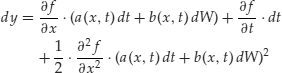
The last expression in parentheses, when expanded, becomes (dropping the arguments of a and b for notational convenience)

To obtain this expression, we dropped the first and the last term in the expanded expression, because they are of order higher than dt. The middle term, , in fact equals b2·dt as dt goes to 0. The latter is not an obvious fact, but it follows from the properties of the standard Wiener process. The intuition behind it is that the variance of (dW)2 is of order dt2, so we can ignore it and treat the expression as deterministic and equal to its expected value. The expected value of (dW)2 is in fact dt.

Substituting this expression back into the expression for dy, we obtain the expression in Ito’s lemma.

Using Ito’s lemma, let us derive the equation for the price at time t, St that was the basis for the exact simulation method for the geometric random walk. Suppose that St follows the GBM

We will use Ito’s lemma to compute the equation for the process followed by the logarithm of the stock price. In other words, in the notation we used in the definition of Ito’s lemma, we have

We also have

Finally, we have

Plugging into the equation for y in Ito’s lemma, we obtain

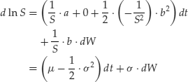
which is the equation we presented earlier. This also explains the presence of the

term in the expression for the drift of the GBM.

KEY POINTS

• Models of asset dynamics include trees (such as binomial trees) and random walks (such as arithmetic, geometric, and mean-reverting random walks). Such models are called discrete when the changes in the asset price are assumed to happen at discrete time increments. When the length of the time increment is assumed to be infinitely small, we refer to them as stochastic processes in continuous time.
• The arithmetic random walk is an additive model for asset prices—at every time period, the new price is determined by the price at the previous time period plus a deterministic drift term and a random shock that is distributed as a normal random variable with mean equal to zero and a standard deviation proportional to the square root of the length of the time period. The probability distribution of future asset prices conditional on a known current price is normal.
• The arithmetic random walk model is analytically tractable and convenient; however, it has some undesirable features such as a nonzero probability that the asset price will become negative.
• The geometric random walk is a multiplicative model for asset prices—at every time period, the new price is determined by the price at the previous time period multiplied by a deterministic drift term and a random shock that is distributed as a lognormal random variable. The volatility of the process grows with the square root of the elapsed amount of time. The probability distribution of future asset prices conditional on a known current price is lognormal.
• The geometric random walk is not only analytically tractable, but is more realistic than the arithmetic random walk, because the asset price cannot become negative. It is widely used in practice, particularly for modeling stock prices.
• Mean reversion models assume that the asset price will meander, but will tend to return to a long-term mean at a speed called the speed of adjustment. They are particularly useful for modeling prices of some commodities, interest rates, and exchange rates.
• The codependence structure between the price processes for different assets can be incorporated directly (by computing the correlation between the random terms in their random walks), by using dynamic multifactor models, or by more advanced means such as copula functions and transfer entropies.
• A variety of more advanced random walk models are used to incorporate different assumptions, such as time-varying volatility and “spikes,” or jumps, in the asset price. They are not as tractable analytically as the classical random walk models, but can be simulated.
• The Wiener process, a stochastic process in continuous time, is a basic building block for many of the stochastic processes used to model asset prices. The increments of a Wiener process are independent, normally distributed random variables with variance proportional to the length of the time period.
• An Ito process is a generalized Wiener process with drift and volatility terms that can be functions of the asset price and time.
• An important result in stochastic calculus is Ito’s lemma, which states that a variable that is a function of a variable that follows an Ito process follows an Ito process itself with specific drift and volatility terms.

REFERENCES

Fabozzi, F. J., Focardi, S., and Kolm, P. N. (2006). Financial Modeling of the Equity Markets: CAPM to Cointegration. Hoboken, NJ: J. Wiley & Sons.

Glasserman, P. (2004). Monte Carlo Methods in Financial Engineering. New York: Springer-Verlag.

Hull, J. (2008). Options, Futures and Other Derivatives, 7th Edition. Upper Saddle River, NJ: Prentice Hall.

Merton, R. C. (1976). Option pricing when underlying stock returns are discontinuous. Journal of Finance, 29: 449–470.

Pachamanova, D. A., and Fabozzi, F. J. (2010). Simulation and Optimization in Finance: Modeling with MATLAB, @RISK, or VBA. Hoboken, NJ: John Wiley & Sons.

Vasicek, O. (1977). An equilibrium characterization of the term structure. Journal of Financial Economics, 5: 177–188.