
When teaching probability, it is customary to give examples of coin tosses. Whether it is going to rain or not is more or less like a coin toss. If we have two possible outcomes, the binomial distribution is appropriate. This distribution requires two parameters: the probability and the sample size.
In statistics, there are two generally accepted approaches. In the frequentist approach, we measure the number of coin tosses and use that frequency for further analysis. Bayesian analysis is named after its founder the Reverend Thomas Bayes. The Bayesian approach is more incremental and requires a prior distribution, which is the distribution we assume before performing experiments. The posterior distribution is the distribution we are interested in and which we obtain after getting new data from experiments. Let's first have a look at the following equations:
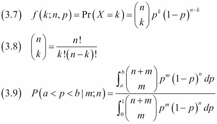
(3.7) and (3.8) describe the probability mass function for the binomial distribution. (3.9) comes from an essay published by Bayes. The equation is about an experiment with m successes and n failures and assumes a uniform prior distribution for the probability parameter of the binomial distribution.
In this recipe, we will apply the frequentist and Bayesian approach to rain data:
- The imports are as follows:
import dautil as dl
from scipy import stats
import matplotlib.pyplot as plt
import numpy as np
from IPython.html.widgets.interaction import interact
from IPython.display import HTML
- Define the following function to load the data:
def load(): rainy = dl.data.Weather.rain_values() > 0 n = len(rainy) nrains = np.cumsum(rainy) return n, nrains - Define the following function to compute the posterior:
def posterior(i, u, data): return stats.binom(i, u).pmf(data[i]) - Define the following function to plot the posterior for the subset of the data:
def plot_posterior(ax, day, u, nrains): ax.set_title('Posterior distribution for day {}'.format(day)) ax.plot(posterior(day, u, nrains), label='rainy days in period={}'.format(nrains[day])) ax.set_xlabel('Uniform prior parameter') ax.set_ylabel('Probability rain') ax.legend(loc='best') - Define the following function to do the plotting:
def plot(day1=1, day2=30): fig, [[upleft, upright], [downleft, downright]] = plt.subplots(2, 2) plt.suptitle('Determining bias of rain data') x = np.arange(n) + 1 upleft.set_title('Frequentist Approach') upleft.plot(x, nrains/x, label='Probability rain') upleft.set_xlabel('Days') set_ylabel(upleft) max_p = np.zeros(n) u = np.linspace(0, 1, 100) for i in x - 1: max_p[i] = posterior(i, u, nrains).argmax()/100 downleft.set_title('Bayesian Approach') downleft.plot(x, max_p) downleft.set_xlabel('Days') set_ylabel(downleft) plot_posterior(upright, day1, u, nrains) plot_posterior(downright, day2, u, nrains) plt.tight_layout() - The following lines call the other functions and place a watermark:
interact(plot, day1=(1, n), day2=(1, n))
HTML(dl.report.HTMLBuilder().watermark())
Refer to the following screenshot for the end result (see the determining_bias.ipynb file in this book's code bundle):

- The Wikipedia page about the essay mentioned in this recipe is at https://en.wikipedia.org/wiki/An_Essay_towards_solving_a_Problem_in_the_Doctrine_of_Chances (retrieved August 2015)