
The Poisson distribution is named after the French mathematician Poisson, who published a thesis about it in 1837. The Poisson distribution is a discrete distribution usually associated with counts for a fixed interval of time or space. It is only defined for integer values k. For instance, we could apply it to monthly counts of rainy days. In this case, we implicitly assume that the event of a rainy day occurs at a fixed monthly rate. The goal of fitting the data to the Poisson distribution is to find the fixed rate.
The following equations describe the probability mass function (3.5) and rate parameter (3.6) of the Poisson distribution:

The following steps fit using the maximum likelihood estimation (MLE) method:
- The imports are as follows:
from scipy.stats.distributions import poisson
import matplotlib.pyplot as plt
import dautil as dl
from scipy.optimize import minimize
from IPython.html.widgets.interaction import interactive
from IPython.core.display import display
from IPython.core.display import HTML
- Define the function to maximize:
def log_likelihood(k, mu): return poisson.logpmf(k, mu).sum() - Load the data and group it by month:
def count_rain_days(month): rain = dl.data.Weather.load()['RAIN'] rain = (rain > 0).resample('M', how='sum') rain = dl.ts.groupby_month(rain) rain = rain.get_group(month) return rain - Define the following visualization function:
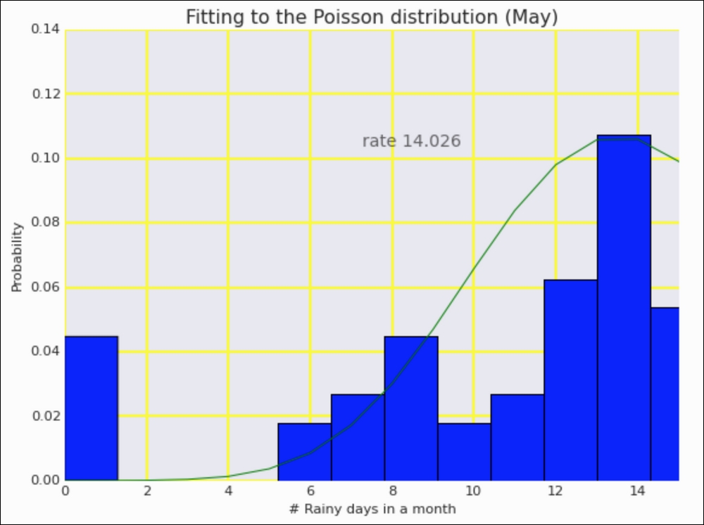
def plot(rain, dist, params, month): fig, ax = plt.subplots() plt.title('Fitting to the Poisson distribution ({})'.format(dl.ts.short_month(month))) # Limiting the x-asis for a better plot plt.xlim([0, 15]) plt.figtext(0.5, 0.7, 'rate {:.3f}'.format(params.x[0]), alpha=0.7, fontsize=14) plt.xlabel('# Rainy days in a month') plt.ylabel('Probability') ax.hist(dist.train, bins=dist.nbins, normed=True, label='Data') ax.plot(dist.x, poisson.pmf(dist.x, params.x)) - Define a function to serve as the entry point:
def fit_poisson(month): month_index = dl.ts.month_index(month) rain = count_rain_days(month_index) dist = dl.stats.Distribution(rain, poisson, range=[-0.5, 19.5]) params = minimize(log_likelihood, x0=rain.mean(), args=(rain,)) plot(rain, dist, params, month_index) - Use interactive widgets so we can display a plot for each month:
display(interactive(fit_poisson, month=dl.nb.create_month_widget(month='May')))
HTML(dl.report.HTMLBuilder().watermark())
Refer to the following screenshot for the end result (see the fitting_poisson.ipynb file in this book's code bundle):
- The Poisson distribution Wikipedia page at https://en.wikipedia.org/wiki/Poisson_distribution (retrieved August 2015)
- The related SciPy documentation at http://docs.scipy.org/doc/scipy/reference/generated/scipy.stats.poisson.html#scipy.stats.poisson (retrieved August 2015)