
Pearson's r, named after its developer Karl Pearson (1896), measures linear correlation between two variables. Let's look at the following equations:
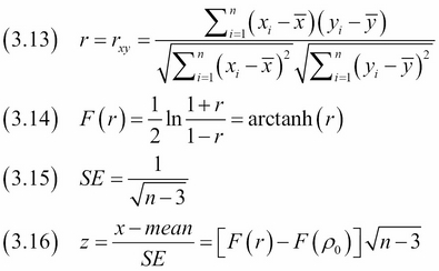
(3.13) defines the coefficient and (3.14) describes the
Fisher transformation used to compute confidence intervals. (3.15) gives the standard error of the correlation. (3.16) is about the z-score of the Fisher transformed correlation. If we assume a normal distribution, we can use the z-score to compute confidence intervals. Alternatively, we can bootstrap by resampling pairs of values with replacement. Also, the scipy.stats.pearsonr() function returns a p-value, which (according to the documentation) is not accurate for samples of less than 500 values. Unfortunately, we are going to use such a small sample in this recipe. We are going to correlate carbon dioxide emission data from the Worldbank with related temperature data for the Netherlands.
In this recipe, we will compute the correlation coefficient and estimate confidence intervals using z-scores and bootstrapping with the following steps:
- The imports are as follows:
import dautil as dl
import pandas as pd
from scipy import stats
import numpy as np
import math
from sklearn.utils import check_random_state
import matplotlib.pyplot as plt
from IPython.display import HTML
from IPython.display import display
- Download the data and set up appropriate data structures:
wb = dl.data.Worldbank() indicator = wb.get_name('co2') co2 = wb.download(country='NL', indicator=indicator, start=1900, end=2014) co2.index = [int(year) for year in co2.index.get_level_values(1)] temp = pd.DataFrame(dl.data.Weather.load()['TEMP'].resample('A')) temp.index = temp.index.year temp.index.name = 'year' df = pd.merge(co2, temp, left_index=True, right_index=True).dropna() - Compute the correlation as follows:
stats_corr = stats.pearsonr(df[indicator].values, df['TEMP'].values) print('Correlation={0:.4g}, p-value={1:.4g}'.format(stats_corr[0], stats_corr[1])) - Calculate the confidence interval with the Fisher transform:
z = np.arctanh(stats_corr[0])
n = len(df.index)
se = 1/(math.sqrt(n - 3))
ci = z + np.array([-1, 1]) * se * stats.norm.ppf((1 + 0.95)/2)

ci = np.tanh(ci)
dl.options.set_pd_options()
ci_table = dl.report.DFBuilder(['Low', 'High'])
ci_table.row([ci[0], ci[1]])
- Bootstrap by resampling pairs with replacement:
rs = check_random_state(34) ranges = [] for j in range(200): corrs = [] for i in range(100): indices = rs.choice(n, size=n) pairs = df.values gen_pairs = pairs[indices] corrs.append(stats.pearsonr(gen_pairs.T[0], gen_pairs.T[1])[0]) ranges.append(dl.stats.ci(corrs)) ranges = np.array(ranges) bootstrap_ci = dl.stats.ci(corrs) ci_table.row([bootstrap_ci[0], bootstrap_ci[1]]) ci_table = ci_table.build(index=['Formula', 'Bootstrap']) - Plot the results and produce a report:
x = np.arange(len(ranges)) * 100
plt.plot(x, ranges.T[0], label='Low')
plt.plot(x, ranges.T[1], label='High')
plt.plot(x, stats_corr[0] * np.ones_like(x), label='SciPy estimate')
plt.ylabel('Pearson Correlation')
plt.xlabel('Number of bootstraps')
plt.title('Bootstrapped Pearson Correlation')
plt.legend(loc='best')
result = dl.report.HTMLBuilder()
result.h1('Pearson Correlation Confidence intervals')
result.h2('Confidence Intervals')
result.add(ci_table.to_html())
HTML(result.html)
Refer to the following screenshot for the end result (see the correlating_pearson.ipynb file in this book's code bundle):

- The related SciPy documentation at http://docs.scipy.org/doc/scipy/reference/generated/scipy.stats.pearsonr.html#scipy.stats.pearsonr (retrieved August 2015).