
Worldwide, there are almost a million dams, roughly 5 percent of which are higher than 15 m. A civil engineer designing a dam will have to consider many factors, including rainfall. Let's assume, for the sake of simplicity, that the engineer wants to know the cumulative annual rainfall. We can also take monthly maximums and fit those to a generalized extreme value (GEV) distribution. Using this distribution, we can then bootstrap to get our estimate. Instead, I select values that are above the 95th percentile in this recipe.
The GEV distribution is implemented in scipy.stats and is a mixture of the Gumbel, Frechet, and Weibull distributions. The following equations describe the cumulative distribution function (3.11) and a related constraint (3.12):
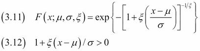
In these equations, μ is the location parameter, σ is the scale parameter, and ξ is the shape parameter.
Let's analyze the data using the GEV distribution:
- The imports are as follows:
from scipy.stats.distributions import genextreme
import matplotlib.pyplot as plt
import dautil as dl
import numpy as np
from IPython.display import HTML
- Define the following function to sample the GEV distribution:
def run_sims(nsims): sums = [] np.random.seed(19) for i in range(nsims): for j in range(len(years)): sample_sum = dist.rvs(shape, loc, scale, size=365).sum() sums.append(sample_sum) a = np.array(sums) low, high = dl.stats.ci(a) return a, low, high - Load the data and select the extreme values:
rain = dl.data.Weather.load()['RAIN'].dropna() annual_sums = rain.resample('A', how=np.sum) years = np.unique(rain.index.year) limit = np.percentile(rain, 95) rain = rain[rain > limit] dist = dl.stats.Distribution(rain, genextreme) - Fit the extreme values to the GEV distribution:
shape, loc, scale = dist.fit() table = dl.report.DFBuilder(['shape', 'loc', 'scale']) table.row([shape, loc, scale]) dl.options.set_pd_options() html_builder = dl.report.HTMLBuilder() html_builder.h1('Exploring Extreme Values') html_builder.h2('Distribution Parameters') html_builder.add_df(table.build()) - Get statistics on the fit residuals:
pdf = dist.pdf(shape, loc, scale) html_builder.h2('Residuals of the Fit') residuals = dist.describe_residuals() html_builder.add(residuals.to_html()) - Get the fit metrics:
table2 = dl.report.DFBuilder(['Mean_AD', 'RMSE']) table2.row([dist.mean_ad(), dist.rmse()]) html_builder.h2('Fit Metrics') html_builder.add_df(table2.build()) - Plot the data and the result of the bootstrap:
sp = dl.plotting.Subplotter(2, 2, context)

sp.ax.hist(annual_sums, normed=True, bins=dl.stats.sqrt_bins(annual_sums))
sp.label()
set_labels(sp.ax)

sp.next_ax()
sp.label()
sp.ax.set_xlim([5000, 10000])
sims = []
nsims = [25, 50, 100, 200]

for n in nsims:
    sims.append(run_sims(n))

sims = np.array(sims)
sp.ax.hist(sims[2][0], normed=True, bins=dl.stats.sqrt_bins(sims[2][0]))
set_labels(sp.ax)

sp.next_ax()
sp.label()
sp.ax.set_xlim([10, 40])
sp.ax.hist(rain, bins=dist.nbins, normed=True, label='Rain')
sp.ax.plot(dist.x, pdf, label='PDF')
set_labels(sp.ax)
sp.ax.legend(loc='best')

sp.next_ax()
sp.ax.plot(nsims, sims.T[1], 'o', label='2.5 percentile')
sp.ax.plot(nsims, sims.T[2], 'x', label='97.5 percentile')
sp.ax.legend(loc='center')
sp.label(ylabel_params=dl.data.Weather.get_header('RAIN'))

plt.tight_layout()
HTML(html_builder.html)
Refer to the following screenshot for the end result (see the extreme_values.ipynb file in this book's code bundle):

- The Wikipedia page on the GEV distribution at https://en.wikipedia.org/wiki/Generalized_extreme_value_distribution (retrieved August 2015).