Conventional shadow mapping renders the scene from the eye and the light, and in the final compositing pass, the two views are compared to identify points that are in shadow [Williams78]. Light-view aliasing results from misalignment of these two views, as shown in Figure 1.6.1(a). There are several variants of shadow mapping that reduce but do not eliminate sampling and self-shadowing artifacts [Fernando01, Stamminger02, Sen03, Lloyd08, Lefohn07], because none of them resolves the fundamental mismatch in sampling patterns between the eye and light views, which is the root cause of most shadow mapping artifacts.

Figure 1.6.1. Conventional versus irregular shadow mapping. In conventional shadow mapping (left), both the eye-view and light-view images are rendered with the classic Z-buffer, leading to a mismatch between the desired and actual sample locations in the shadow map. Irregular shadow mapping (right) avoids this mismatch by rendering the light-view image with the irregular Z-buffer.

Irregular shadow mapping addresses the root cause of visual artifacts in conventional shadow mapping by basing the light-view sampling pattern on the positions of pixels in the eye-view raster and their corresponding depth values, therefore perfectly aligning the compared occluder surface point with the projection of the shadow sample, as illustrated in Figure 1.6.1(b) [Johnson04, Johnson05]. The density of shadow samples varies significantly across the image plane (as seen in Figure 1.6.2), which illustrates the need for an irregular data structure during the light pass.

Figure 1.6.2. The classic Z-buffer (a) samples a scene at regularly spaced points on the light image plane. The irregular Z-buffer (b) samples a scene at arbitrary points on the light image plane. Irregular shadow mapping (d) eliminates aliasing artifacts typically associated with conventional shadow mapping (c).

Irregular shadow mapping utilizes the irregular Z-buffer in this context. This data structure explicitly stores all of the sample locations in a two-dimensional spatial data structure rather than implicitly representing them with a regular pattern. The data structure can be any spatial data structure that supports efficient range queries, such as a k-d tree or a grid. Just as in conventional shadow mapping, irregular shadow mapping projects triangles onto the light-view image plane one at a time and then determines which samples lie inside a triangle. Unlike conventional shadow mapping, this determination is made by querying the irregular Z-buffer. Finally, for each sample inside a triangle, irregular shadow mapping performs the standard depth comparison and updates the sample’s occlusion value.

Note that when a conventional rasterizer is used during light-view projection of occluder triangles, it is necessary to scan-convert expanded triangles to ensure fragments will be generated for any cell touched by the unexpanded triangle (also known as conservative rasterization [Akenine-Möller05]), since irregular Z-buffer samples may lie anywhere within the cell bounds, as illustrated in Figure 1.6.3. For reference, [Hasselgren05] describes a shader implementation with example code. On the other hand, the advantage of a software rasterizer (for example, on Larrabee) is that a special rasterization path can be implemented to apply custom rasterization rules that enable conservative rasterization directly without triangle expansion.

Figure 1.6.3. Conservative rasterization versus conventional rasterization. Scan-converted triangles have to be expanded during light-view projection to ensure fragments will be generated for any cell touched by the unexpanded triangle (shaded cells), since irregular Z-buffer samples (circles) may lie anywhere within the pixel bounds.

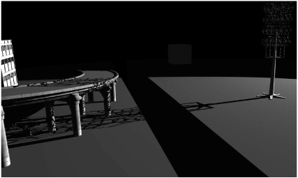
While irregular shadow mapping is free of light-view aliasing, it still suffers from eye-view aliasing of pixels, as illustrated in Figure 1.6.4. Such aliasing is a common problem in computer graphics. For example, it is also encountered in ray casting with a single eye ray per pixel. The problem is that thin geometry (high-frequency screen content) cannot be captured by a single ray, because the rays of two neighboring pixels may miss some geometry even though the geometry projects to part of those pixels. Similarly, in the case of shadows in a rasterizer, it is possible that a surface point projected to the center of an eye-view pixel is lit, but the entire area of the pixel is not lit. This phenomenon, known as eye-view shadow aliasing, is caused by the fact that a single bit occlusion value is not sufficient to represent the occlusion value of aliased pixels. Anti-aliased occlusion values are fractional values that represent the fraction of the total pixel area that is lit. Recently, a few novel shadow mapping techniques [Brabec01, Lauritzen06, Salvi08] have addressed this problem and provide good solutions for eye-view aliasing but still expose light-view aliasing.

Figure 1.6.4. The thin geometry in the tower causes eye-view aliasing of the projected shadow. Note that some of the tower’s connected features are disconnected in the shadow.

The most obvious approach to produce anti-aliased shadows with irregular shadow mapping is super-sampling of the entire screen by generating and evaluating multiple shadow samples for each eye-view pixel. The anti-aliased occlusion value for a pixel is then simply the average of the individual sample occlusion values. While this brute-force approach certainly works, as illustrated in Figure 1.6.5, the computational and storage costs quickly become impractical. Data structure construction, traversal times, and storage requirements of the irregular Z-buffer are proportional to the number of shadow samples, making real-time performance impossible on current hardware for even as little as four shadow samples per pixel.

Figure 1.6.5. A four-times super-sampled irregular shadow mapping result image of the tower scene.

The recent method by [Robison09] provides a solution to compute anti-aliased shadows from the (aliased) output of irregular shadow mapping, but in essence it is also a brute-force approach in screen space that does not exploit the irregular Z-buffer acceleration structure and is therefore at a computational disadvantage compared to our approach.

We will now give an overview of the complete algorithm to provide structure to the remainder of the algorithm description in this section. Then we describe how to determine which pixels are potentially aliased by constructing a conservative shadow edge stencil buffer and how to splat multiple samples into the irregular Z-buffer efficiently. Finally, we put it all together and present the complete algorithm in practice.

We can formulate our approach in the following top-level description of our algorithm:

To adaptively add shadow samples at shadow-edge pixels, we construct a special stencil buffer that answers the following question: Is there any chance that this eye-space pixel is partially occluded by geometry in this light-space texel? We call this stencil buffer the conservative shadow edge stencil buffer. Giving an exact answer to the aforementioned question is impossible because it is essentially solving the shadowing problem. However, we can use a probabilistic technique to answer the question conservatively with sufficient confidence. A conservative answer is sufficient for our purpose, since multi-sampling of non-shadow-edge pixels does not alter the correctness of the result—it only adds some extra cost. Obviously, we strive to make the stencil buffer only as conservative as necessary.

We employ a technique called Variance Shadow Mapping [Lauritzen06]. Variance shadow maps encode a distribution of depths at each light-space texel by determining the mean and variance of depth (the first two moments of the depth distribution). These moments are constructed through mip-mapping of the variance shadow map. When querying the variance shadow map, we use these moments to compute an upper bound on the fraction of the distribution that is more distant than the surface being shaded, and therefore this bound can be used to cull eye-view pixels that have very little probability to be in shadow.

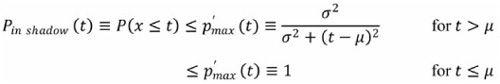
In particular, the cumulative distribution function F(t) = P(x ≥ t) can be used as a measure of the fraction of the eye-view fragment that is lit, where t is the distance of the eye-view sample to the light, x is the occluder depth distribution, and P stands for the probability function. While we cannot compute this function F(t) exactly, Chebyshev’s inequality gives an upper bound:

The upper bound P_max (t) and the true probability P_lit (t) are depicted in Figure 1.6.6. Thus, we can determine that it is almost certain that a projected eye-view sample with light depth t is in shadow (for example, with 99-percent certainty) by comparing P_max to 1% (P_max < implies P_lit (t) < 0.01).

Figure 1.6.6. P_{in shadow} (t) and P_lit (t), in addition to their conservative upper bounds P_max (t) and p′_max (t).

Conversely, we can use the same distribution to construct a bound to cull eye-view pixels that have very high probability of being lit:

In summary, the conservative shadow edge stencil buffer can be constructed in the following steps:

These steps can be implemented in HLSL shader pseudocode, as shown in Listing 1.6.1.

float2 ComputeMoments(float Depth)
{
    // Compute first few moments of depth
    float2 Moments;
    Moments.x = Depth;
    Moments.y = Depth * Depth;
    return Moments;
}

float ChebyshevUpperBound(
  float2 moments, float mean, float minVariance)
{
    // Compute variance
    float variance = max(
               minVariance,
               moments.y - (moments.x * moments.x));
    float d        = mean - moments.x;
    float pMax     = variance / (variance + (d * d));

    // One-tailed Chebyshev's Inequality
    return (mean <= moments.x ? 1.0f : pMax);
}

bool IsPotentialShadowEdge(float2 texCoord,
                           float2 texCoordDX,
                           float2 texCoordDY,
                           float  depth)
{
    float4 occluderData;
    // Variance Shadow Map mip-mapped LOD tex lookup
    occluderData = texShadowMap.SampleGrad(
      sampShadowMap,
      texCoord, texCoordDX, texCoordDY);

    float2 posMoments = occluderData.xy;

    // Minimum variance to take account for variance
    // across entire pixel
    float gMinVariance = 0.000001f;

    float pMaxLit = ChebyshevUpperBound(
        posMoments, depth, gMinVariance);
    float pMaxShadow = ChebyshevLowerBound(
        posMoments, depth, gMinVariance);

    if (PMaxLit < .01 || PMaxShadow < .01) {
      return true;
    }

    return false;
}

Note that while conventional rasterization of the scene from the light’s point of view in Step 1 earlier is sufficient for generating a conventional variance shadow map, it is not sufficient for generating our conservative stencil buffer. Conventional rasterization does not guarantee that a primitive’s depth contributes to the minimum depth of each light-view texel that it touches. Hence, the conservativeness of the stencil buffer would not be preserved as illustrated in Figure 1.6.7, which depicts potential shadow-edge pixels in overlay but misses quite a few due to the low resolution of the variance shadow map.

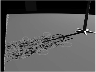
Figure 1.6.7. Conservative shadow edge stencil map with regular rasterization. Many potential shadow-edge pixels (overlay) are missed due to low resolution of the variance shadow map.

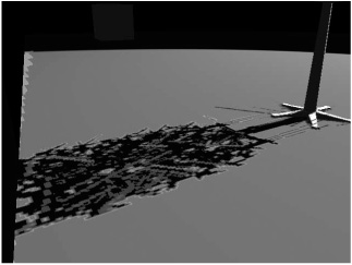
To preserve conservativeness, it is required to perform conservative rasterization in the light-view render of Step 1, just as we do during the light-view render of irregular shadow mapping illustrated in Figure 1.6.3. Figure 1.6.8 depicts correctly detected potential shadow-edge pixels in overlay, regardless of the variance shadow map resolution.

Figure 1.6.8. Conservative shadow edge stencil map with conservative rasterization. All potential shadow-edge pixels are detected (overlay), regardless of the variance shadow map resolution.

In the irregular Z-buffer construction phase, when the time comes to generate additional samples for potentially aliased pixels, as defined by the conservative shadow edge stencil buffer, we insert the eye-view samples in each light-view grid cell that is touched by the pixel samples. We call this process shadow sample splatting, because we conceptually splat the projection of the pixel footprint into the light space grid data structure. This process is as follows:

On Larrabee, we have implemented Steps 2 and 3 of our algorithm in an efficient post-process over all eye-view pixels in parallel. However, Step 3 is identical to the conventional irregular shadowing algorithm; therefore, it could be implemented as in [Arvo07] as well.

Conceptually, we use a grid-of-lists representation for the irregular Z-buffer. This representation is well-suited to parallel and streaming computer architectures and produces high-quality shadows in real time in game scenes [Johnson05]. The following chapter of this book [Hux10], in particular Figure 1.7.1, explains our grid-of-lists representation and its construction in more detail.

Finally, our solution was implemented in a deferred renderer, but it could also be implemented in a forward renderer with a few modifications.

Since only a marginal fraction of all screen pixels are shadow-edge pixels, this approach results in substantial gains in computational and storage costs compared to the brute-force approach. Compared to the single-sample irregular shadow maps, the additional computational cost is relatively small. For example, let’s assume the number of potential shadow-edge pixels is ~10 percent of all eye-view pixels, and that we generate N additional samples per potential shadow-edge pixel. Since data structure construction and traversal times are proportional to the number of shadow map samples, this means an additional cost of 10N percent for anti-aliasing.

Additionally, there is an extra cost associated with creating the conservative shadow edge stencil buffer. In our implementation inside a deferred rendering, much of the required information was already computed—therefore, that extra cost is small. However, our algorithm does require an extra light-space pass, per light, to capture the depth distribution into the variance shadow map.

The storage cost is the same as the standard irregular Z-buffer, proportional to the number of samples. Again, for 10-percent extra samples, 10N-percent extra storage is required, depending on the implementation. Storage of the stencil buffer requires only 1 bit per eye-view pixel and can easily be packed into one of the existing eye-view buffers of the irregular shadowing algorithm.

Going forward, we would like to investigate the benefits of merging our algorithm that adaptively samples potential shadow edge pixels multiple times with conventional multi-sampling techniques that adaptively sample the geometry silhouette pixels multiple times—for best performance, preferably through the use of common data structures and shared rendering passes. Additionally, it should be fairly straightforward to extend our approach to soft irregular shadow mapping, where the concept of anti-aliasing is implicit, as both the soft and hard irregular shadow mapping algorithms share the same algorithmic framework [Johnson09]. For soft shadows, one may envision extending the conservative stencil to shadow penumbra detection.