What is needed is a way to structure the scene so that we can quickly and easily determine whether a given surface point is occluded by nearby geometry. It turns out that the standard depth buffer, which graphics engines already use to perform hidden surface removal, can be used to approximate local occlusion [Shanmugam07, Mittring07]. By definition, the depth buffer contains the depth of every visible point in the scene. From these depths, we can reconstruct the 3D positions of the visible surface points. Points that can potentially occlude other points are located close to each other in both screen space and world space, making the search for potential occluders straightforward. We need to align a hemisphere around each point’s upper hemisphere as defined by its normal. We will thus need a normal buffer that will encode the normal of every corresponding point in the depth buffer in screen space.

Rather than doing a full ray intersection, we can simply inspect the depths of neighboring points to establish the likelihood that each is occluding the current point. Any neighbor whose 2D position does not fall within the 2D coverage of the hemisphere could not possibly be an occluder. If it does lie within the hemisphere, then the closer the neighbor point’s depth is to the target point, the higher the odds it is an occluder. If the neighbor’s depth is behind the point being tested for occlusion, then no occlusion is assumed to occur. All of these calculations can be performed using the screen space buffer of normals and depths, hence the name Screen Space Ambient Occlusion (SSAO).

At first glance, this may seem like a gross oversimplification. After all, the depth buffer doesn’t contain the whole scene, just the visible parts of it, and as such is only a partial reconstruction of the scene. For example, a point in the background could be occluded by an object that is hidden behind another object in the foreground, which a depth buffer would completely miss. Thus, there would be pixels in the image that should have some amount of occlusion but don’t due to the incomplete representation we have of the scene’s geometry.

Figure 1.2.2. SSAO Samples neighbor points to discover the likelihood of occlusion. Lighter arrows are behind the center point and are considered occluded samples.

It turns out that these kinds of artifacts are not especially objectionable in practice. The eye focuses first on cues from objects within the scene, and missing cues from objects hidden behind one another are not as disturbing. Furthermore, ambient occlusion is a low-frequency phenomenon; what matters more is the general effect rather than specific detailed cues, and taking shortcuts to achieve a similar yet incorrect effect is a fine tradeoff in this case. Discovering where the artifacts lie should be more a process of rationalizing the errors than of simply catching them with the untrained eye.

From this brief overview, we can outline the steps we will take to implement Screen Space Ambient Occlusion.

I will now describe our Screen Space Ambient Occlusion algorithm in greater detail.

The first step in setting up the SSAO algorithm is to prepare the necessary incoming data. Depending on how the final compositing is to be done, this can be accomplished in one of two ways.

The first method requires that the scene be rendered twice. The first pass will render the depth and normal data only. The SSAO algorithm can then generate the ambient occlusion output in an intermediate step, and the scene can be rendered again in full color. With this approach, the ambient occlusion map (in screen space) can be sampled by direct lights from the scene to have their contribution modulated by the ambient occlusion term as well, which can help make the contributions from direct and indirect lighting more coherent with each other. This approach is the most flexible but is somewhat less efficient because the geometry has to be passed to the hardware twice, doubling the API batch count and, of course, the geometry processing load.

A different approach is to render the scene only once, using multiple render targets bound as output to generate the depth and normal information as the scene is first rendered without an ambient lighting term. SSAO data is then generated as a post-step, and the ambient lighting term can simply be added. This is a faster approach, but in practice artists lose the flexibility to decide which individual lights in the scene may or may not be affected by the ambient occlusion term, should they want to do so. Using a fully deferred renderer and pushing the entire scene lighting stage to a post-processing step can get around this limitation to allow the entire lighting setup to be configurable to use ambient occlusion per light.

Whether to use the single-pass or dual-pass method will depend on the constraints that are most important to a given graphics engine. In all cases, a suitable format must be chosen to store the depth and normal information. When supported, a 16-bit floating-point format will be the easiest to work with, storing the normal components in the red, green, and blue components and storing depth as the alpha component.

Screen Space Ambient Occlusion is very bandwidth intensive, and minimizing sampling bandwidth is necessary to achieve optimal performance. Moreover, if using the single-pass multi-render target approach, all bound render targets typically need to be of the same bit depth on the graphics hardware. If the main color output is 32-bit RGBA, then outputting to a 16-bit floating-point buffer at the same time won’t be possible. To minimize bandwidth and storage, the depth and normal can be encoded in as little as a single 32-bit RGBA color, storing the x and y components of the normal in the 8-bit red and green channels while storing a 16-bit depth value in the blue and alpha channels. The HLSL shader code for encoding and decoding the normal and depth values is shown in Listing 1.2.1.

// Normal encoding simply outputs x and y components in R and G in
// the range 0.. 1
float3 DecodeNormal( float2 cInput ) {
     float3 vNormal.xy = 2.0f * cInput.rg - 1.0f;
     vNormal.z = sqrt(max(0, 1 - dot(vNormal.xy, vNormal.xy)));
     return vNormal;
}

// Encode depth to B and A
float2 DepthEncode( float fDepth ) {
    float2 vResult;
    // Input depth must be mapped to 0..1 range
    fDepth = fDepth / p_fScalingFactor;

    // R = Basis = 8 bits = 256 possible values
    // G = fractional part with each 1/256th slice
    vResult.ba = frac( float2( fDepth, fDepth * 256.0f ));
    return vResult;
}

float3 DecodeDepth( float4 cInput ) {
    return dot ( cInput.ba, float2( 1.0f, 1.0f / 256.0f ) *
                 p_fScalingFactor;
}

With the input data in hand, we can begin the ambient occlusion generation process itself. At any visible point on a surface on the screen, we need to explore neighboring points to determine whether they could occlude our current point. Multiple samples are thus taken from neighboring points in the scene using a filtering process described by the HLSL shader code in Listing 1.2.2.

// i_VPOS is screen pixel coordinate as given by HLSL VPOS interpolant.
// p_vSSAOSamplePoints is a distribution of sample offsets for each sample.
float4 PostProcessSSAO( float 3 i_VPOS )
{
   float2 vScreenUV;       //←This will become useful later.
   float3 vViewPos = 2DToViewPos( i_VPOS, vScreenUV);

   half fAccumBlock = 0.Of;
   for (inti = 0; i < iSampleCount; i++ )
   {
       float3 vSamplePointDelta = p_vSSAOSamplePoints[i];
       float fBlock = TestOcclusion(
                          vViewPos,
                             vSamplePointDelta,
                          p_fOcclusionRadius,
                          p_fFullOcclusionThreshold,
                          p_fNoOcclusionThreshold,
                          p_fOcclusionPower ) )
       fAccumBlock += fBlock;
   }
   fAccumBlock / = iSampleCount;

   return 1.Of - fAccumBlock;
}

We start with the current point, p, whose occlusion we are computing. We have the point’s 2D coordinate in screen space. Sampling the depth buffer at the corresponding UV coordinates, we can retrieve that point’s depth. From these three pieces of information, the 3D position of the point within can be reconstructed using the shader code shown in Listing 1.2.3.

// vRecipDepthBufferSize = 1.0 / depth buffer width and height in pixels.
// p_vCameraFrustrumSize = Full width and height of camera frustum at the
// camera's near plane in world space.
float2 p_vRecipDepthBufferSize;
float2 p_vCameraFrustrumSize;
float3 2DPosToViewPos( float3 i_VPOS, out float2 vScreenUV )
{
    float2 vViewSpaceUV = i_VPOS * p_vRecipDepthBufferSize;
    vScreenUV    = vViewSpaceUV;

    // From 0..1 to to 0..2
    vViewSpaceUV = vViewSpaceUV * float2( 2.Of, -2.Of );
    // From 0..2 to-1..1
    vViewSpaceUV = vViewSpaceUV + float2( -1.0f , 1.Of );
    vViewSpaceUV = vViewSpaceUV * p_vCameraFrustrumSize * 0.5f;

    return float3( vViewSpaceUV.x, vViewSpaceUV.y, 1.0f ) *
                   tex2D( p_sDepthBuffer, vScreenUV ).r;
}

We will need to sample the surrounding area of the point p along multiple offsets from its position, giving us n neighbor positions qi. Sampling the normal buffer will give us the normal around which we can align our set of offset vectors, ensuring that all sample offsets fall within point p’s upper hemisphere. Transforming each offset vector by a matrix can be expensive, and one alternative is to perform a dot product between the offset vector and the normal vector at that point and to flip the offset vector if the dot product is negative, as shown in Figure 1.2.3. This is a cheaper way to solve for the offset vectors without doing a full matrix transform, but it has the drawback of using fewer samples when samples are rejected due to falling behind the plane of the surface of the point p.

Figure 1.2.3. Samples behind the hemisphere are flipped over to stay within the hemisphere.

Each neighbor’s 3D position can then be transformed back to screen space in 2D, and the depth of the neighbor point can be sampled from the depth buffer. From this neighboring depth value, we can establish whether an object likely occupies that space at the neighbor point. Listing 1.2.4 shows shader code to test for this occlusion.

float TestOcclusion( float3 vViewPos,
                     float3 vSamplePointDelta,
               float fOcclusionRadius,
                     float fFullOcclusionThreshold,
                     float fNoOcclusionThreshold,
   float fOcclusionPower )
{
    float3 vSamplePoint = vViewPos + fOcclusionRadius * vSamplePointDelta;
    float2 vSamplePointUV;
    vSamplePointUV = vSamplePoint.xy / vSamplePoint.z;
    vSamplePointUV = vSamplePointUV / p_vCameraSize / 0.5f;
    vSamplePointUV = vSamplePointUV + float2( 1.0f, -1.0f );
    vSamplePointUV = vSamplePointUV * float2( 0.5f, -0.5f );

    float fSampleDepth = tex2D( p_sDepthBuffer, vSamplePointUV ).r;
    float fDistance = vSamplePoint.z - fSampleDepth;
    return OcclusionFunction( fDistance, fFullOcclusionThreshold,
                              fNoOcclusionThreshold, fOcclusionPower );
}

We now have the 3D positions of both our point p and the neighboring points qi. We also have the depth di of the frontmost object along the ray that connects the eye to each neighboring point. How do we determine ambient occlusion?

The depth di gives us some hints as to whether a solid object occupies the space at each of the sampled neighboring points. Clearly, if the depth di is behind the sampled point’s depth, it cannot occupy the space at the sampled point. The depth buffer does not give us the thickness of the object along the ray from the viewer; thus, if the depth of the object is anywhere in front of p, it may occupy the space, though without thickness information, we can’t know for sure. We can devise some reasonable heuristics with the information we do have and use a probabilistic method.

The further in front of the sample point the depth is, the less likely it is to occupy that space. Also, the greater the distance between the point p and the neighbor point, the lesser the occlusion, as the object covers a smaller part of the hemisphere. Thus, we can derive some occlusion heuristics based on:

For the first relationship, we can formulate an occlusion function to map the depth deltas to occlusion values.

If the aim is to be physically correct, then the occlusion function should be quadratic. In our case we are more concerned about being able to let our artists adjust the occlusion function, and thus the occlusion function can be arbitrary. Really, the occlusion function can be any function that adheres to the following criteria:

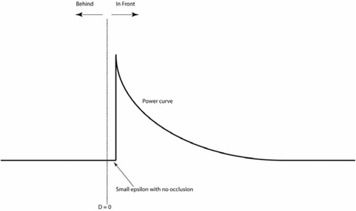
For our implementation, we simply chose a linearly stepped function that is entirely controlled by the artist. A graph of our occlusion function is shown in Figure 1.2.4. There is a full-occlusion threshold where every positive depth delta smaller than this value gets complete occlusion of one, and a no-occlusion threshold beyond which no occlusion occurs. Depth deltas between these two extremes fall off linearly from one to zero, and the value is exponentially raised to a specified occlusion power value. If a more complex occlusion function is required, it can be pre-computed in a small ID texture to be looked up on demand.

Figure 1.2.4. SSAO blocker function.

float OcclusionFunction( float fDistance,
                         float fNoOcclusionThreshold,
float fFullOcclusionThreshold,
float fOcclusionPower )
{
    const c_occlusionEpsilon = 0.01f;

    if ( fDistance > c_ occlusionEpsilon )
    {
        // Past this distance there is no occlusion.
        float fNoOcclusionRange = fNoOcclusionThreshold -
                                  fFullOcclusionThreshold;
        if ( fDistance < fFullOcclusionThreshold )
            return 1.0f;
        else return max(1.0f – pow(( ( fDistance –
             fFullOcclusionThreshold ) / fNoOcclusionRange,
             fOcclusionPower ) ) ,0.0f );
    } else return 0.0f;
}

Once we have gathered an occlusion value for each sample point, we can take the average of these, weighted by the distance of each sample point to p, and the average will be our ambient occlusion value for that pixel.

Sampling neighboring pixels at regular vector offsets will produce glaring artifacts to the eye, as shown in Figure 1.2.5.

Figure 1.2.5. SSAO without random sampling.

To smooth out the results of the SSAO lookups, the offset vectors can be randomized. A good approach is to generate a 2D texture of random normal vectors and perform a lookup on this texture in screen space, thus fetching a unique random vector per pixel on the screen, as illustrated in Figure 1.2.6 [Mittring07]. We have n neighbors we must sample, and thus we will need to generate a set of n unique vectors per pixel on the screen. These will be generated by passing a set of offset vectors in the pixel shader constant registers and reflecting these vectors through the sampled random vector, resulting in a semi-random set of vectors at each pixel, as illustrated by Listing 1.2.6. The set of vectors passed in as registers is not normalized—having varying lengths helps to smooth out the noise pattern and produces a more even distribution of the samples inside the occlusion hemisphere. The offset vectors must not be too short to avoid clustering samples too close to the source point p. In general, varying the offset vectors from half to full length of the occlusion hemisphere radius produces good results. The size of the occlusion hemisphere becomes a parameter controllable by the artist that determines the size of the sampling area.

Figure 1.2.6. Randomized sampling process.

float3 reflect( float 3 vSample, float3 vNormal )
{
      return normalize ( vSample – 2.0f * dot( vSample, vNormal ) * vNormal );
}

float3x3 MakeRotation( float fAngle, float3 vAxis )
{
    float fS;
    float fC;
    sincos( fAngle, fS, fC );
    float fXX       = vAxis.x * vAxis.x;
    float fYY       = vAxis.y * vAxis.y;
    float fZZ       = vAxis.z * vAxis.z;
    float fXY       = vAxis.x * vAxis.y;
    float fYZ       = vAxis.y * vAxis.z;
    float fZX       = vAxis.z * vAxis.x;
    float fXS       = vAxis.x * fS;
    float fYS       = vAxis.y * fS;
    float fZS       = vAxis.z * fS;
    float fOneC      = 1.0f - fC;

    float3x3 result = float3x3(
        fOneC * fXX +  fC,  fOneC * fXY + fZS, fOneC * fZX - fYS,
        fOneC * fXY - fZS,  fOneC * fYY +  fC, fOneC * fYZ + fXS,
        fOneC * fZX + fYS,  fOneC * fYZ - fXS, fOneC * fZZ +  fC
    );
    return result;
}

float4 PostProcessSSAO( float3 i_VPOS )
{

      ...

      const float c_scalingConstant = 256.0f;
      float3 vRandomNormal = ( normalize( tex2D( p_sSSAONoise, vScreenUV *
                                                      p_vSrcImageSize / c_scalingConstant ).xyz * 2.0f
                                                      – 1.0f ) );
      float3x3 rotMatrix = MakeRotation( 1.0f,vNormal );

      half fAccumBlock = 0.0f;
      for ( int i = 0; i < iSampleCount; i++ ) {
          float3 vSamplePointDelta = reflect( p_vSSAOSamplePoints[i],
                                                                 vRandomNormal );
          float fBlock = TestOcclusion(
                             vViewPos,
      vSamplePointDelta,
                             p_fOcclusionRadius,
                             p_fFullOcclusionThreshold,
                             p_fNoOcclusionThreshold,
                             p_fOcclusionPower ) ) {
       fAccumBlock += fBlock;
      }

     ...

}

As shown in Figure 1.2.7, the previous step helps to break up the noise pattern, producing a finer-grained pattern that is less objectionable. With wider sampling areas, however, a further blurring of the ambient occlusion result becomes necessary. The ambient occlusion results are low frequency, and losing some of the high-frequency detail due to blurring is generally preferable to the noisy result obtained by the previous steps.

Figure 1.2.7. SSAO term after random sampling applied. Applying blur passes will further reduce the noise to achieve the final look.

To smooth out the noise, a separable Gaussian blur can be applied to the ambient occlusion buffer. However, the ambient occlusion must not bleed through edges to objects that are physically separate within the scene. A form of bilateral filtering is used. This filter samples the nearby pixels as a regular Gaussian blur shader would, yet the normal and depth for each of the Gaussian samples are sampled as well. (Encoding the normal and depth in the same render targets presents significant advantages here.) If the depth from the Gaussian sample differs from the center tap by more than a certain threshold, or the dot product of the Gaussian sample and the center tap normal is less than a certain threshold value, then the Gaussian weight is reduced to zero. The sum of the Gaussian samples is then renormalized to account for the missing samples.

// i_UV : UV of center tap
// p_fBlurWeights Array of gaussian weights
// i_GaussianBlurSample: Array of interpolants, with each interpolants
// packing 2 gaussian sample positions.
float4 PostProcessGaussianBlur( VertexTransport vertOut )
{
     float2 vCenterTap    = i_UV.xy;
     float4 cValue        = tex2D( p_sSrcMap, vCenterTap.xy );
     float4 cResult       = cValue * p_fBlurWeights[0];
     float fTotalWeight   = p_fBlurWeights[0];

     // Sample normal & depth for center tap
     float4 vNormalDepth = tex2D( p_sNormalDepthMap, vCenterTap.xy ).a;
     for ( int i = 0; i < b_iSampleInterpolantCount; i++ )
     {
         half4 cValue = tex2D( p_sSrcMap,
                               i_GaussianBlurSample[i].xy );
         half fWeight = p_fBlurWeights[i * 2 + 1];

         float4 vSampleNormalDepth = tex2D( p_sNormalDepthMap,
                                     i_GaussianBlurSample[i].xy );
         if ( dot( vSampleNormalDepth.rgb, vNormalDepth.rgb) < 0.9f ||
              abs( vSampleNormalDepth.a – vNormalDepth.a ) > 0.01f )
             fWeight = 0.0f;

         cResult += cValue * fWeight;
         fTotalWeight += fWeight;

         cValue = tex2D( p_sSeparateBlurMap,
                         INTERPOLANT_GaussianBlurSample[i].zw ) ;
         fWeight = p_fBlurWeights[i * 2 + 2];
         vSampleNormalDepth = tex2D( p_sSrcMap,
                              INTERPOLANT_GaussianBlurSample[i].zw ) ;
         if ( dot( vSampleNormalDepth.rgb, vNormalDepth .rgb < 0.9f ) ||
                   abs( vSampleNormalDepth.a – vNormalDepth.a ) > 0.01f )
              fWeight = 0.0f;
         cResult += cValue * fWeight;
         fTotalWeight += fWeight;
     }

     // Rescale result according to number of discarded samples.
     cResult *= 1.0f / fTotalWeight;

     return cResult;
}

Several blur passes can thus be applied to the ambient occlusion output to completely eliminate the noisy pattern, trading off some higher-frequency detail in exchange.

Figure 1.2.8. Result of Gaussian blur.

The offset vectors are in view space, not screen space, and thus the length of the offset vectors will vary depending on how far away they are from the viewer. This can result in using an insufficient number of samples at close-up pixels, resulting in a noisier result for these pixels. Of course, samples can also go outside the 2D bounds of the screen. Naturally, depth information outside of the screen is not available. In our implementation, we ensure that samples outside the screen return a large depth value, ensuring they would never occlude any neighboring pixels. This can be achieved through the “border color” texture wrapping state, setting the border color to a suitably high depth value.

To prevent unacceptable breakdown of the SSAO quality in extreme close-ups, the number of samples can be increased dynamically in the shader based on the distance of the point p to the viewer. This can improve the quality of the visual results but can result in erratic performance. Alternatively, the 2D offset vector lengths can be artificially capped to some threshold value regardless of distance from viewer. In effect, if the camera is very close to an object and the SSAO samples end up being too wide, the SSAO area consistency constraint is violated so that the noise pattern doesn’t become too noticeable.

Screen Space Ambient Occlusion can have a significant payoff in terms of mood and visual quality of the image, but it can be quite an expensive effect. The main bottleneck of the algorithm is the sampling itself. The semi-random nature of the sampling, which is necessary to minimize banding, wreaks havoc with the GPU’s texture cache system and can become a problem if not managed. The performance of the texture cache will also be very dependent on the sampling area size, with wider areas straining the cache more and yielding poorer performance. Our artists quickly got in the habit of using SSAO to achieve a faked global illumination look that suited their purposes. This required more samples and wider sampling areas, so extensive optimization became necessary for us.

One method to bring SSAO to an acceptable performance level relies on the fact that ambient occlusion is a low-frequency phenomenon. Thus, there is generally no need for the depth buffer sampled by the SSAO algorithm to be at full-screen resolution. The initial depth buffer can be generated at screen resolution, since the depth information is generally reused for other effects, and it potentially has to fit the size of other render targets, but it can thereafter be downsampled to a smaller depth buffer that is a quarter size of the original on each side. The downsampling itself does have some cost, but the payback in improved throughput is very significant. Downsampling the depth buffer also makes it possible to convert it from a wide 16-bit floating-point format to a more bandwidth-friendly 32-bit packed format.

If the ambient occlusion hemisphere is large enough, the SSAO algorithm eventually starts to mimic behavior seen from general global illumination; a character relatively far away from a wall could cause the wall to catch some of the subtle shadowing cues a global illumination algorithm would detect. If the sampling area of the SSAO is wide enough, the look of the scene changes from darkness in nooks and crannies to a softer, ambient feel.

This can pull the art direction in two somewhat conflicting directions: on the one hand, the need for tighter, high-contrast occluded zones in deeper recesses, and on the other hand, the desire for the larger, softer, ambient look of the wide-area sampling.

One approach is to split the SSAO samples between two different sets of SSAO parameters: Some samples are concentrated in a small area with a rapidly increasing occlusion function (generally a quarter of all samples), while the remaining samples use a wide sampling area with a gentler function slope. The two sets are then averaged independently, and the final result uses the value from the set that produces the most (darkest) occlusion. This is the approach that was used in StarCraft II.

Figure 1.2.9. SSAO with different sampling-area radii.

The edge-enhancing component of the ambient occlusion does not require as many samples as the global illumination one, thus a quarter of the samples can be assigned to crease enhancement while the remainder are assigned for the larger area threshold.

Though SSAO provides for important lighting cues to enhance the depth of the scene, there was still a demand from our artist for more accurate control that was only feasible through the use of some painted-in ambient occlusion. The creases from SSAO in particular cannot reach the accuracy that using a simple texture can without using an enormous amount of samples. Thus the usage of SSAO does not preclude the need for some static ambient occlusion maps to be blended in with the final ambient occlusion result, which we have done here.

Figure 1.2.10. Combined small- and large-area SSAO result.

For our project, complaints about image noise, balanced with concerns about performance, were the main issues to deal with for the technique to gain acceptance among our artists. Increasing SSAO samples helps improve the noise, yet it takes an ever-increasing number of samples to get ever smaller gains in image quality. Past 16 samples, we’ve found it’s more effective to use additional blur passes to smooth away the noise pattern, at the expense of some loss of definition around depth discontinuities in the image.

It should be noted the depth buffer can only contain one depth value per pixel, and thus transparencies cannot be fully supported. This is generally a problem with all algorithms that rely on screen space depth information. There is no easy solution to this, and the SSAO process itself is intensive enough that dealing with edge cases can push the algorithm outside of the real-time realm. In practice, for the vast majority of scenes, correct ambient occlusion for transparencies is a luxury that can be skimped on. Very transparent objects will typically be barely visible either way. For transparent objects that are nearly opaque, the choice can be given to the artist to allow some transparencies to write to the depth buffer input to the SSAO algorithm (not the z-buffer used for hidden surface removal), overriding opaque objects behind them.

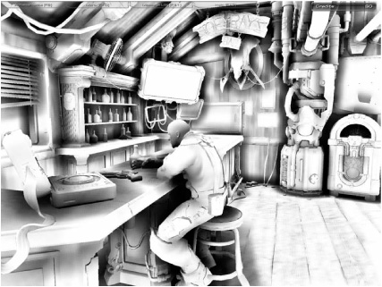
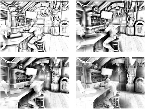
Color Plate 1 shows some results portraying what the algorithm contributes in its final form. The top-left pane shows lighting without the ambient occlusion, while the top-right pane shows lighting with the SSAO component mixed in. The final colored result is shown in the bottom pane. Here the SSAO samples are very wide, bathing the background area with an effect that would otherwise only be obtained with a full global illumination algorithm. The SSAO term adds depth to the scene and helps anchor the characters within the environment.

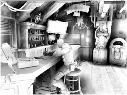
Color Plate 2 shows the contrast between the large-area, low-contrast SSAO sampling component on the bar surface and background and the tighter, higher-contrast SSAO samples apparent within the helmet, nooks, and crannies found on the character’s spacesuit.

This gem has described the Screen Space Ambient Occlusion technique used at Blizzard and presented various problems and solutions that arise. Screen Space Ambient Occlusion offers a different perspective in achieving results that closely resemble what the eye expects from ambient occlusion. The technique is reasonably simple to implement and amenable to artistic tweaks in real time to make it ideal to fit an artistic vision.