
Simon Schirm and Mark Harris, NVIDIA Corporation
[email protected], [email protected]
Over the past several years, physically based simulation has become an important feature of games. Effects based on physical simulation of phenomena such as liquid, smoke, particulate debris, cloth, and rigid body dynamics greatly increase the level of realism and detail in a game. These effects can be expensive to simulate using traditional sequential approaches, especially in a complex game engine where the CPU is already handling many expensive tasks. On the other hand, there is a lot of data parallelism in many physical simulations, and the GPUs in most modern PCs and consoles are powerful parallel processors that can be applied to this task. Simulating fluids and particles on the GPU enables games to incorporate complex fluids and particle effects with tens of thousands of particles that interact with the player and the game scenery.
NVIDIA PhysX is a real-time physics engine for games that uses the GPU in concert with the CPU to accelerate physically based simulation of particle systems, fluids, cloth, and rigid body dynamics [NVIDIA09a]. The GPU-accelerated portions of the engine are implemented using the C for CUDA language and the CUDA run-time API. The standard C and C++ language support in the CUDA compiler makes programming, debugging, and maintaining the complex algorithms used in PhysX much easier and ensures that they can be integrated efficiently with the CPU portions of the engine. For more information on CUDA, see [NVIDIA09b].
In this gem, we present the algorithms and implementation details for the particle and fluid systems in PhysX. We describe the features of each system and then present an overview of the algorithm and details of the implementation in CUDA. Figure 7.3.1 and Color Plate 15 are examples of the results of the techniques described in this gem.
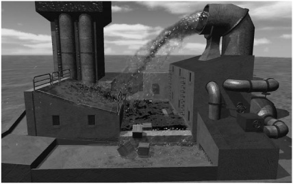
Figure 7.3.1. Real-time GPU-accelerated Smoothed Particle Hydrodynamics (SPH) water simulation in PhysX. There are more than 60,000 particles in the simulation. The rendering is performed using a screen-space splatting technique.
Particle systems are ubiquitously used in games to create a variety of effects. Particles can be used to represent media ranging from highly granular materials, such as leaves, gravel, and sparks, to more continuous media, such as smoke or steam. Particle effects in games are typically tailored to interact as lightly as possible with the scene in order to reduce computational overhead. This is done, for example, by applying pre-computed forces to the particles in a way that doesn’t require any intersection tests or collision detection. The range of effects that can be achieved is therefore significantly limited. One goal of PhysX is to relax these restrictions by moving expensive but highly parallel calculations to the GPU, enabling particles to interact with geometrically rich and dynamic scenes.
Real-time simulation of fluids can dramatically increase the realism and interactivity of smoke, steam, and liquid effects in games. The PhysX SDK supports the simulation of gaseous and liquid fluids by adding support for particle-particle interactions to its particle systems. Inter-particle forces are defined so that the volume the particles occupy is approximately conserved over time.
PhysX fluid simulation is built on top of the particle system component, sharing the same collision algorithm and spatial partitioning data structure. Like particle systems, fluid motion is not practically limited to a box domain; particles and fluids can spread throughout a game level.
PhysX particles are allowed to interact with arbitrary triangle meshes in a game scene, and therefore we need an algorithm that can robustly handle particle collisions with these meshes. This is particularly challenging in the presence of inter-particle forces, which tend to literally push particles into all the edge and corner cases. Our algorithm has the following properties.
Penetration and artificial energy loss are minimized so that particles don’t leak or stick as shown in Figure 7.3.2: Left.
A configurable collision radius is provided.
High-velocity collisions are handled. (The collision radius is usually small compared to the distance a fast particle travels per time step.)
Particles on thin static objects cannot be pushed through by dynamic objects penetrating the static geometry, as shown in Figure 7.3.2: Right.

The PhysX particle collision algorithm is based on a mixed approach that makes use of both continuous and discrete collision detection, as illustrated in Figure 7.3.3.

Right: A discrete collision detection test between a particle and geometry.
Figure 7.3.3. Left: Continuous collision detection (CCD) with multiple shapes.
The linear path of the particle motion is tested for intersection with any dynamic or static objects in order to find the first impact location. For dynamic objects, the intersection test must be handled with extra care. Each particle’s original position p is transformed into the local space of the moving object according to its original pose. The target position q is correspondingly transformed according to the target pose of the object, as shown in Figure 7.3.4. Now the linear path defined by the transformed local positions p’ and q’ is tested against the object in its local space. This is just an approximation, since the motion path of the particle observed from the moving dynamic geometry would generally be curved. Nonetheless, this approximation has the nice property that the test is topologically correct when multiple compound geometries are involved. Practically, this means that a particle-filled hollow box doesn’t leak particles when shaken.

Right: The same situation as on the left, but relative to a moving shape. Instead of intersecting the curved particle path, a linear approximation is used.
Figure 7.3.4. Left: Continuous collision detection with a dynamic shape.
In addition to the continuous collision test, the sphere defined by the target particle position and radius is tested for intersections with nearby geometry, as shown in Figure 7.3.3: Right. Both results are combined to calculate an appropriate collision response for the particle.
The collision algorithm must gracefully handle cases in which particles could get trapped between penetrating scene objects, as shown in Figure 7.3.2: Right. In practice, it makes sense to give collisions with static objects precedence over collisions with dynamic objects. This is achieved by dividing the collision algorithm into a first pass handling dynamic objects and a second pass handling static objects.
Particles are often continuously pushed against scene geometry by gravity or fluid forces. In these cases, the particle path intersects close to the particle’s current position. Correct continuous collision detection will prevent a particle from sliding along object boundaries. One way to overcome this is to correct the velocity of the particle and check its new path for potential collisions again for the rest of the time step. This can be repeated until the end of the time step is reached and the final position of the particle is found. For a particle in a corner, this iteration might take forever. To solve this problem, our algorithm remembers the surfaces a particle collided with in the previous time step and uses them in the current time step to correct the particle velocity in a pre-process to collision detection. In practice, it turns out that storing two planes— called surface constraints—per particle is enough to provide good results in most cases.
To simulate a fluid, one must compute the mass (and other field values) carried by the fluid through space over time. There are two fundamental approaches to fluid simulation:
Eulerian simulations track fluid field values at fixed locations in space—for example, on a grid.
Lagrangian simulations track fluid field values at locations moving with the flow—for example, by using particles.
In PhysX, using particles has several advantages.
Particles are already used in games, which eases the integration.
Particles enable seamless collisions with static geometry and rigid bodies with no boundary resampling.
Mass conservation is trivially achieved by associating a constant mass with each particle.
The approach we use in PhysX is called Smoothed Particle Hydrodynamics (SPH), which is a Lagrangian simulation technique that was originally developed to simulate the motion of galaxies [Monaghan92] and later applied to free-surface fluid flow simulation. SPH is an interpolation method that allows field values that are defined only at particle positions to be evaluated anywhere in space [Müller03]. The method is based on the Navier-Stokes equations, which describe fluid motion by relating continuous velocity, density, and pressure fields over time. The two equations enforce conservation of mass and momentum. Since mass is conserved by using discrete particles, we only use the momentum equation. In Lagrangian form, it reads as follows:
All terms in Equation (1) are derived from local field properties at the location xi of particle i. The mass of each particle is constant over time. ![]() represents the acceleration of the particle, and the three terms on the right-hand side describe contributions to the acceleration.
represents the acceleration of the particle, and the three terms on the right-hand side describe contributions to the acceleration.
External acceleration g, including gravity and collision impulses.
Force due to the fluid pressure gradient ▽p|xi.
Force due to the viscosity of the fluid, given by the Laplacian of the velocity field ▽2v|xi weighted by the scalar viscosity of the fluid μ.
The pressure and viscosity terms each represent a so-called “body force,” which is a force per unit volume. To convert a body force into acceleration using Newton’s second law, it must be normalized by the mass density ρi at the location of the particle, as shown in Equation (1).
The particles act as sample points for the continuous physical fields. Radially symmetric kernel functions are used to reconstruct smooth fields from the discrete particle samples, hence the name Smoothed Particle Hydrodynamics.
To evaluate a field value at a certain location, the contributions of the overlapping kernel functions at each nearby particle are summed up, as shown in Figure 7.3.5. Correspondingly, the pressure gradient and the velocity Laplacian can be derived using the kernel functions, as described by [Müller03]. Choosing kernels with a finite non-zero domain is crucial to accelerating the search for nearby particles.

Figure 7.3.5. A one-dimensional field reconstruction formed by the summation of overlapping kernels for each particle.
To compute the acceleration on each particle in the fluid, we need to evaluate Equation (1) at the particle position by summing up the kernel contributions from all overlapping particles. In practice, this requires evaluating three physical fields: density, pressure, and viscosity. This can be done in two passes: one to evaluate the density field and another to evaluate pressure and viscosity, which both depend on density. After evaluating Equation (1) in this way, we have an acceleration that can be used to integrate the velocity and position of the particle over the time step.
For further details on SPH and our application of the method, see [Müller03].
Figure 7.3.6 shows an overview of the fluid simulation pipeline. First, the spatial domain that is covered by the particles is approximated with a set of bounds. These are inserted into the broad phase along with the bounds of static and dynamic objects in the scene. In parallel with the broad phase, the SPH phase computes fluid forces and uses them to update the particle velocity. The particle collision phase uses the output of the broad phase and the SPH phase to compute collisions with dynamic and static objects and applies velocity impulses to resolve any penetration. Finally, the positions of all particles are updated using their newly computed velocities.

To support efficient collision detection between particles and static geometry and rigid bodies present in the scene, we need to avoid testing all possible particle-object pairs for intersections. The so-called broad phase collision detection algorithm compares the spatial bounds of scene objects to find all potentially colliding pairs. Checking the bounds of all individual particles would overload the broad phase. Therefore, we generate bounds for groups of spatially coherent particles. The particles are associated with a particular particle group based on a hash grid similar to the one used for finding neighbors in SPH but with much coarser grid spacing. The particle collision algorithm uses the output of the broad phase, a set of pairs of overlapping particle groups and scene objects, to find the intersections of individual particles with scene objects. The broad phase can run in parallel in a separate CPU thread while the GPU executes the SPH phase, since the result of the broad phase is only needed before the collision phase starts.
The SPH phase computes the density and force at each particle position xi. The force computation evaluates the influence of all other particles in a neighborhood around xi. In order to find neighboring particles efficiently, we use a hashed regular grid to accelerate finding nearby particles. A hashed grid implementation similar to the one used in PhysX is demonstrated in the “particles” sample in the NVIDIA CUDA SDK [Green09], as described by [Teschner03].
Building the hashed grid data structure requires two steps. The first step computes a hash index for each particle such that all particles in the same grid cell have the same hash index. The second step sorts all particle data by hash index so that the data for all particles in the same hash cell is contiguous in memory.
To compute the hash index, each particle position (x, y, z) is discretized onto a virtual (and infinite) 3D grid by dividing its coordinates by the grid cell size and rounding down to the nearest integer coordinates (i, j, k) = ([x/h], [y/h], [z/h]). These coordinates are then used as input to a hash function that computes a single integer hash index. Our hash function is simple; it computes the integer coordinates modulo the grid size and linearizes the resulting 3D coordinates, as shown in Listing 7.3.1. This simple hash function has the important property that given a hash index, computing the hash indices of neighboring cells is trivial, because neighboring cells in the virtual grid map to neighboring cells in the hash grid (modulo the grid size).
Example 7.3.1. The virtual grid hash function. Note that GRID_SIZE must be a power of 2.
int3 gridPosition(float3 pos, float cellSize)
{

   int3 gridPos;
   gridPos.x = floor(pos.x/cellSize) & (GRID_SIZE – 1);
   gridPos.y = floor(pos.y/cellSize) & (GRID_SIZE – 1);
   gridPos.z = floor(pos.z/cellSize) & (GRID_SIZE – 1);
   return gridPos;
}
int hash(int3 gridPos)
{
   return (gridPos.z * GRID_SIZE + gridPos.y) * GRID_SIZE + gridPos.x;
}
The hash values for each particle are computed in a CUDA C kernel that outputs an array of hash indices and an array of corresponding particle indices. These are then used as arrays of keys and corresponding indices, which we sort using the fast CUDA radix sort of [Satish09]. For each hash grid cell, we also store the sorted indices of the first and last particle in the cell, to enable constant-time queries of the particles in each hash cell. After the key-index pairs are sorted, we use the sorted indices to reorder the particle position and velocity arrays. Reordering the data arrays is important because it ensures efficient, coalesced memory accesses in subsequent CUDA computations.
Using parallel sorting to build this “list of lists” grid structure is more efficient than building it directly (in other words, by appending each particle to a list for each grid cell) in parallel, because we don’t know a priori which cells are occupied and how many particles are in each cell. An advantage of using a radix sort is that multiple non-interacting fluids can be combined within the same virtual grid at low additional cost, because doubling the number of fluids only adds one bit to the sort key length. We simply process the particles of all fluids together in parallel and append the fluid ID above the most significant bit of the hash index. Then when we sort the particles, they will be sorted first by fluid ID and then by hash index. This enables us to do all subsequent steps in the simulation of all fluids in parallel. To reduce sorting cost, we sort using only as many bits as we need to represent our chosen grid resolution, which currently is log2 Nf + 18 bits (64×64×64 grid), where Nf is the number of fluids.
With the use of a hash, we can handle an unlimited grid. Therefore, the fluid is not confined to a box but can flow anywhere in the scene. Naturally, in a widely dispersed fluid, particles from far-apart cells may hash to the same index. If many non-interacting particles hash to the same index, we will perform unnecessary work to evaluate their Euclidean distance, but in practice this has not been a problem. For more on evaluating hash functions and hash table size, see [Teschner03].
Once the hashed grid is built, it can be used to quickly find all particles near to each particle. Thus, we can evaluate the density and force by finding the cell each particle resides in and iterating over the 27 neighboring cells in 3D. At each neighboring cell, we perform a hash table lookup to find the list of particles in each cell. Using these particles, we can compute the sum of the influences of each neighboring particle, as shown in Listing 7.3.2.
Example 7.3.2. Pseudocode for evaluating a smoothing kernel at a particle’s position
SumOfSupportFunctions(float3 pos, float cellSize)
{

   int3 gridPos = gridPosition(pos, cellSize);
   for (int i = -1; i <= 1; i++)
      for (int j = -1; j <= 1; j++)
         for (int k = -1; k <= 1; k++) {
             gridPosition += int3(i, j, k);
             particles = hashTableLookup(hash(gridPosition))
             foreach particle p in particles {
                sum += supportFunction(pos, p.position);
             }
         }
}
The procedure in Listing 7.3.2 can be applied to both of the steps required to compute the body forces in Equation (1). First, it is used to compute density using the density kernel function. Then, the density is used to compute pressure and viscosity using the pressure and viscosity kernel functions. For details of these kernel functions, see [Müller03].
The four SPH steps shown in Figure 7.3.6 are implemented using one CUDA C kernel each to compute the particle hash, the density, and the force at each particle, plus a radix sort, which is implemented using multiple CUDA C kernels as described in [Satish09], and a kernel that finds the starting and ending indices of particles in each cell and reorders the particle position and velocity arrays using the sorted indices.
The particle hash kernel simply computes the hash index for each particle given its 3D position using the function in Listing 7.3.1. We launch as many GPU threads as there are particles in the scene and compute one hash per thread. After sorting the particles by hash index using the radix sort, we launch another kernel, again with one thread per particle, to reorder the particle position and velocity arrays. This kernel also compares each particle’s hash index against those before and after it in the sorted array. If it is different from the index before it, then we know this is the first particle in a cell, so we store this particle’s index in the sorted array to a “cell starts” array at the cell index. If it is different from the index after it, then it is the end of a cell, so we store its index in a “cell ends” array.
The density and force kernels also process one particle per thread. Each thread runs the procedure given in Listing 7.3.2. The density kernel uses the density support function given in [Müller03] as its support function to compute a scalar density per particle. The force kernel computes two 3D force sums, one using the pressure gradient support function and one using the viscosity Laplacian support function, both given in [Müller03]. The hashTableLookup function in Listing 7.3.2 simply reads the indices at the cell’s index in the cell start and cell end arrays to get a range of particle indices to read from the sorted particle position and velocity arrays.
We make several optimizations to our CUDA C kernels to ensure best performance. First, we pack together the data for all active particle systems or fluids into large batches so that the CUDA kernels can process all particles at once. This improves utilization of the GPU in the presence of multiple small particle systems. We add a small amount of padding between the end of one particle system’s data and the beginning of the next to ensure that each particle system begins on an aligned boundary, and we use structures of arrays (SOA) rather than arrays of structures for the particle data. This means that instead of having an array of particle structures containing particle position, velocity, and other data, we have an array of all particle positions, an array of all velocities, and so on. These optimizations ensure that parallel thread accesses to the data arrays are coalesced by the GPU [NVIDIA09b]. Finally, the density and force kernels bind a texture reference to the data arrays so that the spatially coherent but non-sequential access pattern of these kernels can benefit from the texture cache hardware on the GPU [NVIDIA09b].
The collision phase uses the particle positions and updated velocities from the SPH phase (which includes external accelerations, such as gravity) to compute intersections with scene geometry and rigid bodies and to prevent penetration. The collision algorithm is composed of the following sequence of stages:
Within each stage we can treat particles independently, and therefore we typically use one CUDA thread per particle. The particle data as well as any temporary per-particle storage is laid out as structures of arrays (SOA) for efficient coalesced memory access. As with the SPH stage, in order to improve the utilization of the GPU, each CUDA kernel processes multiple particle systems together in one batch.
The first collision CUDA kernel loads up to two surface constraints from the previous time step for each particle, if available. From the current particle position and velocity, we compute a target position. The target position is projected out of the surface to get a motion path that is not in conflict with the surface the particle is in contact with. The target position is then passed on to the next stage.
Intersection tests for static and dynamic shapes can be handled with the same set of CUDA kernels, treating a static shape as a special case of a dynamic shape that doesn’t move. The collision detection described in this section is therefore executed twice— first for dynamic shapes and then for static shapes.
For each spatially coherent group of particles, we need to find all relevant intersections with all shapes that are provided by the broad phase for this group. To improve execution coherence on the data-parallel GPU architecture, we run a different CUDA kernel for each shape type. Our collision algorithm handles collisions with capsules, convex meshes, and triangle mesh shape types, so we have three shape-specific collision kernels.
Each shape-specific kernel iterates over its shapes by looping over batches of shape data (capsule extents and radii, triangles, or planes depending on shape type) that are loaded by all threads cooperatively from global device memory into fast on-chip shared memory. Then, for each loaded batch, each thread tests one particle for intersection with all shapes in the batch and aggregates the contact information.
In the case of triangle meshes, an additional optimization improves GPU utilization when there are more triangles than particles in the spatial group. Instead of using one thread per particle, it is more efficient to parallelize across triangles (in other words, run one thread per triangle). However, since particles may collide with multiple triangles, we would need to store contact information per particle-triangle pair, which is not memory efficient. Our approach is to perform parallel early-out tests for which the results (one bit per test) can be stored very efficiently. This is done as follows. For each triangle, all particles are investigated to find the ones that potentially collide, ruling out the others with a relatively cheap conservative intersection test. The per-particle contact generation can then skip triangles for which the early-out test had a negative result.
After the dynamic shape collision detection, a CUDA kernel computes a collision response from the aggregated surface contact information and updates particle target positions accordingly. After the static shape collision detection, the collision response kernel is executed again, providing the final particle position.
Displaying materials in games that are represented as particles requires very different approaches depending on the material. Granular materials, such as gravel, leaves, or sparks, can be rendered using instanced meshes or billboard techniques, such as impostors. Gaseous fluids are typically displayed using a billboard per particle and various blending methods. Adding environmental shadowing and self-shadowing improves the realism with some added performance cost. The “Smoke Particles” sample in the NVIDIA CUDA SDK demonstrates this technique [Green09]. Rendering liquids based on particle simulation is particularly challenging, since a smooth surface needs to be extracted.
Extracting a surface from a set of points is typically done using the grid-based marching cubes algorithm [Lorensen87], which creates the surface by marching through voxels and generating triangles in cells through which an isosurface is found to pass. This method, however, doesn’t provide real-time performance for the resolution and particle count we are targeting. A real-time alternative is the approach described by [Müller07], which simplifies the marching cubes to marching squares to generate a surface mesh in screen space. A further simplification is to avoid any polygonization of the surface and work entirely at the pixel level. This is the approach used in the demo shown in Figure 7.3.1 [NVIDIA08].
Our screen-space rendering approach is as follows.
Render the scene to a color texture and to the depth buffer.
Render all particles to a depth texture as sphere point sprites.
Render the particle thickness to a “thickness” texture with additive blending.
Smooth the depth texture to avoid a “particle appearance.”
Compute a surface normal texture from the smoothed depth using central differencing.
Use the normal, depth, and thickness to render the fluid surface into the scene color texture with proper depth testing, reflection, refraction, and Fresnel term.
These steps are all implemented in a standard graphics API using pixel and vertex shaders. The smoothing step is very important; without it, the fluid will look like a collection of discrete particles. There are multiple ways to implement this smoothing. The basic approach used in Figure 7.3.1 is to smooth the depth texture using a separable Gaussian blur filter. This is inexpensive but can lead to a somewhat “blobby” appearance. A more sophisticated approach is to apply curvature flow, as described by [van der Laan09]. Their technique achieves much more smoothing in areas of low curvature, while maintaining sharp details. A comparison of the two techniques is shown in Color Plate 16.
We measured the performance of the PhysX particle fluid demo shown in Figure 7.3.1 and Color Plate 16 on a PC with Intel Core 2 Quad CPU and an NVIDIA GeForce GTX 260 GPU. The demo was run with a screen resolution of 1024×768 and an average of about 60,000 particles. Figure 7.3.7 presents the results. The time taken for rendering and CUDA kernels in PhysX is about balanced; on the other hand, the PhysX SDK work executed on the CPU contributes relatively strongly. This can be improved by moving all of the per-particle processing onto the GPU. The executions of the CUDA kernels take 8.2 ms on average. For SPH, the summation passes over particle neighbors that compute density and force take most of the time. For collision, the largest portion is contributed from collisions with the static triangle mesh.

The CUDA fluid simulation implementation and the ideas behind it are the fruits of the efforts of a large team. We would like to thank all the members of the NVIDIA PhysX team and others at NVIDIA for their contributions, especially Steve Borho, Curtis Davis, Stefan Duthaler, Isha Geigenfeind, Monier Maher, Simon Green, Matthias Müller-Fischer, Ashu Rege, Miguel Sainz, Richard Tonge, Lihua Zhang, and Jiayuan Zhu. We would also like to thank Gareth Ramsey and Eidos Game Studios for the use of Color Plate 15.