Often, the method for classifying errors in integration techniques is to label them as first order, second order, and so on. Methods that are first order have an upper bound error on the order of the time step taken to the first power. Methods that are second order have an upper bound error on the order of the time step to the second power. Taking a small number to a large power makes the small number smaller. Thus, higher-order methods yield more accuracy.

Error can also be classified in terms of how well an integrator conserves energy. Integrators might add or remove energy from the system. Some integrators can conserve energy on average. For instance, the semi-implicit, or Symplectic Euler, method is a first-order method, but it conserves energy on average. If an integrator adds energy to the system, the system can become unstable and diverge, especially at higher time steps. The accuracy of a method can affect its stability, but it does not determine it, as shown by the Symplectic Euler method. More often than not, it is the stability of a method that we desire, more than the accuracy.

In this gem we will be taking a different approach to classifying error. This approach is based on the fact that the stepping equations usually assume that the acceleration is constant over the course of a time step. The kinematics of constant acceleration are a problem that can be solved easily and exactly. Comparing the kinematic equations of constant acceleration with the results of a numerical method provides qualitative insight into sources of error in the method.

When derivatives are discretized, it is done by means of a finite difference. Such a finite difference of positions implies that the velocity is constant over the course of the time step. In order to introduce a non-constant velocity, you must explicitly introduce an equation involving acceleration. Similarly, the only way to deal with non-constant acceleration is to explicitly introduce an equation involving the derivative of acceleration. Since many numerical methods do not involve any such equation, we are safe in making the comparison with the kinematic equations for constant acceleration, at least over the course of a single time step.

We know the exact form of the trajectory of particles that are subject to a constant acceleration.

We can compare this set of equations to the results of common numerical methods in order to gain a qualitative idea about the error in the method. Consider the standard Euler method:

v_n+1 = v_n + a_n Δ t

x_n+1 = x_n + v_n Δ t

This set of equations can be transformed into a set that more closely resembles the kinematic equations by inserting the velocity equation into the position equation:

v_n+1 = v_n + a_n Δ t

x_n+1 = x_n + v_n-1 Δ t + a_n-1 Δ t²

The appearance of v_n-1 in the position equation is due to the fact that we must insert v_n and must therefore re-index the velocity equation. The differences in form of this equation to the kinematic equations can be considered as qualitatively representative of the error of the method.

We may perform this same procedure with the Symplectic Euler method:

v_n+1 = v_n + a_n Δ t

x_n+1 = x_n + v_n+1 Δ t

Insert the velocity equation into the position equation to transform to the kinematic form:

v_n+1 = v_n + a_n Δ t

x_n+1 = x_n + v_n Δ t + a_n Δ t²

This equation is a much closer match in form to the kinematic equations. We can use this resemblance to justify the fact that the Symplectic Euler method must in some way be better than the standard Euler method.

If we are trying to find an integration method that when converted to a kinematic form is identical to the kinematic equations, why not just use the kinematic equations as the integration method?

If we do this, then we are guaranteed to get trajectories that are exact, within the assumption that acceleration is constant over the course of the time step. However, the accelerations we are usually interested in modeling are not constant over the course of the time step. We must use a value for the acceleration that encapsulates the fact that the acceleration is changing.

We could use the acceleration averaged over the time step, , as the constant acceleration value. By inserting the average acceleration into the kinematic equations, we achieve a method that we will refer to as the average acceleration method. In order to calculate this average exactly, we must analytically integrate the acceleration over the time step, which in many instances can be done easily. The average acceleration method therefore represents a blend between numerical and analytic integration. We are numerically integrating the current position and velocity from the previous position and velocity, but we are analytically integrating accelerations that are acting during the current time step.

Of course, calculating the average acceleration exactly requires that we know how to integrate the particular force in question. Luckily, most forces that are applied in game physics are analytic models that are easily integrated. Calculating the average acceleration from an analytic model of a force is usually just as easy as calculating the acceleration at an instant of time.

If the average acceleration is calculated analytically, then the velocity portion of the kinematic equations produces exact results. However, the position portion would require a double integral in order to achieve an exact result. If the forces that we are dealing with follow simple analytic models, then calculating a double integral is usually just as easy as calculating a single integral.

We will generalize the idea of the average acceleration method in order to introduce the kinematic integrator. The kinematic integrator is a set of stepping equations that allow for exact analytic calculation of both the velocity integral and the position integral.

v_n+1 = v_n + dv

x_n+1 = x_n + v_n Δ t + dx

The exact method uses the following definitions for dv and dx:

If we are using the average acceleration method, then we define dv and dx as:

In the case of constant acceleration, it is very easy to perform both the single and the double integral. The integral contributions of a constant acceleration are given as:

If there are multiple forces acting on a body, we can express the integral contributions as a sum of contributions that are due to each force.

dv = dv₁ + dv₂ + …

dx = dx₁ + dx₂ + …

Thus for the kinematic integrator we accumulate dv’s and dx’s rather than accelerations. All forces acting on a body provide contributions to dv and dx. The amount that is contributed is dependent on the nature of the force and can usually be calculated exactly. If all forces acting on a body are integrable, then every contribution is exact.

The kinematic integrator can be used to perform the Symplectic Euler method with the following integral contributions:

dv = a_n Δ t

dx = a_n Δ t²

This method is useful if the acceleration is not integrable (or if we are too lazy to calculate the integrals). These contributions are not going to be exact, but they will at least conserve energy, which will maintain stability.

The kinematic integrator does not represent a specific integration method, but rather the ability to isolate the portions of the stepping equations that actually require integration. Since the method used to evaluate the integral contributions is not explicitly specified, we have a degree of freedom in choosing which method might be best for a particular force. For instance, if there is a contribution from a constant gravitational force, then we can easily use the exact method. We will see that for some forces we will want to use the average acceleration method. Or we could use the Symplectic Euler method if the force in question is too complicated to integrate or if we are performing a first pass on the implementation of a particular force.

Probably one of the most common forces, next to a constant uniform force, is a spring force. The spring force is proportional to the displacement of the spring from equilibrium. This results in the following equation of motion:

The solution of this equation of motion is analytically solvable and is given by:

x – l = A cos (ωt) + B sin(ωt)

v = –A sin(ωt) + ωB cos(ωt)

Using this exact trajectory, we can determine the integral contributions:

where c and s represent the cosine and sine, respectively, of ω(t). We could represent this calculation as a matrix operation.

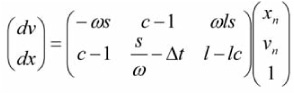
The components of this matrix depend on the size of the time step Δt, the mass of the body m, the strength of the spring k, and the equilibrium position of the spring l. The components of the matrix can be cached and reused until any of these parameters change. In many instances, these parameters do not change for the lifetime of the spring. Thus, the calculation of the integral contributions of a spring is relatively trivial—in other words, six multiplies and four adds.

We can consider that the spring that we have been discussing is anchored to an infinitely rigid object at the origin, since we have only taken into account the action of the spring on a single body, and the spring coordinates are the same as the body coordinates. It is only slightly more complicated to calculate the integral contributions due to a spring that connects two movable bodies.

Before discussing the integral contributions of other possible forces, we need to discuss what happens when multiple forces act on a body.

If all of the forces acting on a body depend only on time, then the result of accumulating exact integral contributions will be exact. But consider the case where at least one of the forces depends on the position of the body, such as the spring force.

The integral contribution of the spring takes into account the position of the body at intermediate values as the spring acts over the course of the time interval. However, the calculation is not aware of intermediate changes in position that are due to other forces. The result is a very slight numerical error in the resulting trajectory of the particle.

As an example, consider two springs that are acting on the same body. For simplicity, both springs are attached to an infinitely rigid body at the origin, and the rest length of both springs is zero. The springs have spring constants k₁ and k₂. The acceleration becomes:

a = –(ω₁)² x – (ω₂)²x

If we are to handle these forces separately, then we would exactly calculate the integral contributions of two springs, with frequencies ω₁ and ω₂, and accumulate the results.

The springs can also be combined into a single force.

In this case, only a single integral contribution would be calculated. It might be surprising to discover that these two methods produce different results. The second method is exact, while the first contains a slight amount of numerical error. This seems to imply that:

∫(a₁ + a₂)dt ≠ ∫ a₁dt + ∫ a₂dt

which is usually not true. However, in the current circumstance, if the acceleration is a function of the position, which in turn is a function of the acceleration, then the integrals have feedback. The effect of this feedback is that we cannot separate the sum into independent integrals, since the independent integrals will not receive feedback from each other.

If the acceleration only depends on time, there is no feedback, and the integrals can safely be separated. Because of this, you may want to separate out forces that depend only on time and accumulate their integral contributions as a group. The integral contributions of these forces can be safely added together without introducing numerical error. Unfortunately, most of the forces that are applicable to game physics depend on the position of the body.

Though the error due to multiple forces is incredibly small, it represents a tiny violation of energy conservation. If this violation persists for long enough, then the trajectory can eventually diverge. The error due to multiple forces is initially much less than the error in the Symplectic Euler method, but it can eventually grow until it is out of control.

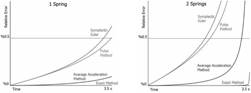
Since we can integrate exactly the system with two springs, we can use this example to gauge the error present in the different methods for calculating the integral contributions. Results of this error calculation are contained in the figures. The first figure contains the results of integrating one spring; the second figure represents errors due to integrating two springs. The integration takes place over one half of the period of the two-spring system.

The Symplectic Euler method as well as the pulse method (which will be introduced later) both conserve energy on average. Neither the average acceleration method nor the exact method conserve energy over long intervals of time. It takes quite a while, but the exact method will eventually diverge. The average acceleration method will eventually dampen out. For this reason, the average acceleration method is preferred if the integration is going to take place over a long interval.

Figure 2.5.1. The relative errors in the case of one spring and two springs.

One solution to the problem due to multiple forces is to approximate the action of the force as a pulse. A pulse is a force that acts very briefly over the course of the time step. A perfect pulse acts instantaneously. Pulses acting at the beginning of the time step do not depend on intermediate values of position or velocity; therefore, pulses are immune to the multiple-force problems.

Consider a rectangular pulse. The area under the curve of a rectangular pulse is dv = adt, where dt is the width of the pulse, and a is the magnitude of the pulse. It is possible to shrink the width of the pulse while maintaining the same area. To do this, we must, of course, increase the magnitude of the pulse. If we allow the pulse width to go to zero, the height diverges to infinity. However, the product of the width and the height is still equal to dv. In the case where dv = 1, there is a special name for this infinite pulse. It is called a delta function, and is denoted as δ(t). The delta function is zero at all values of t, except at t = 0. At t = 0, the delta function is equal to infinity. Integrating the delta function is very easy to do.

for all values of a and b where a < 0 < b. If the interval between a and b does not contain zero, then the result of the integral is zero.

To represent the force as a pulse, we define the acceleration as:

a = dvδ(t)

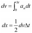
Here, dv is the area under the curve of this instantaneous pulse, as previously described. Integrating this acceleration is easy to do:

∫ adt = dv

Integrating the position contribution is now just integrating a constant.

We can choose dv as the amount of acceleration we want to pack into the pulse. If we want to pack all of the acceleration due to an arbitrary force into the pulse, then we use the average value of the acceleration . This produces stepping equations of the form: In a more familiar form, the stepping equations for the pulse would appear as:

In a more familiar form, the stepping equations for the pulse would appear as:

If you make the assumption that the acceleration is constant over the time interval, then you can replace with a_n. Doing this, you will arrive back at the stepping equations for the standard Symplectic Euler method. This gives meaningful insight into the Symplectic Euler method. It is a method that assumes that the acceleration is constant over the course of the time step and delivers all of the acceleration in an instantaneous pulse at the beginning of the time step. Since pulses can be accumulated without introducing error, the Symplectic Euler method can be considered to be an exact solution to forces of an approximated form. Since the method is exact, it intrinsically conserves energy. The error in the method is entirely due to the differences between the actual form of the force and the approximate form of the pulse.

One very common thing that needs to be done in a game physics engine is to resolve collisions. To calculate our collision, we will assume that the forces due to the collision act within some subinterval that fits entirely within our given time interval. The nature of the force does not matter as much as the fact that it operates on a very small timescale and achieves the desired result.

For simplicity, we will assume that the object has normal incidence with a plane boundary. We will also assume that the collision with the boundary is going to take place within the time interval.

To handle the collision correctly, we should sweep the trajectory of the body between x_n and x_n+1 and find the exact position and the exact time where the collision begins to take place. If we want to find the projected position at the next time step x_n+1, we should wait to apply the collision force until all other forces have been applied, so that the projected next position is as accurate as possible.

For the purpose of simplification, we will consider that the trajectory is a straight line that connects the position x_n with x_n+1. The position of the body at some intermediate value of the time step is given by:

X_f = X_n(1–f)+X_n+1(f)

where f is the fraction of the time step that represents the moment of impact. The intermediate velocity is simplified as well, to be:

V_f = V_n(1–f)+V_n+1(f)

With this physically inaccurate yet simplified trajectory, we can perform a sweep of the body against the collision boundary. The result of this sweep will determine the time fraction f. This will tell us the position and velocity (almost) of the body at the moment of impact. To determine the force that is applied in order to resolve the collision, we need to apply a pulse force that reflects the component of velocity v_f about the contact plane. This reflection incorporates the interaction of the body with the contact surface; thus, the result should incorporate surface friction. For now, we will assume that there is no friction.

To apply the pulse force, we will begin by applying a constant force over a small subinterval of the time step. The subinterval begins at time fΔt and ends at (f + df)Δt. The velocity of the body at the end of the subinterval is given by:

v_{f + df} = v_f + a_vdf

According to our initial simplification, the velocity is aligned with the normal of the contact plane. Thus, all of the velocity is reflected. We choose a_v to enact this reflection.

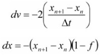
The integral contributions of this force in the limit that df → 0 are given by:

dv_v – 2v_f

dx_v = 0

Since this force pulse does not contribute anything to the position integral, the application of this force does not change the value of x_n+1 from what it would have been. Thus, the value of x_n+1 will still violate the collision constraint.

We need to apply a second force pulse, which moves the position of the body out of the collision surface. Assuming that the body has normal incidence to the plane, then the amount the body needs to be pushed is given by Δx = x_f – x_n+1. Again, we are going to apply a constant force on a subinterval. The acceleration of this force a_x is determined by considering the kinematic equations for constant acceleration.

The integral contributions for this acceleration as df → 0 are:

Adding these two sets of contributions together gives the final result for the collision force. This set of contributions can be expressed in terms of the position at the beginning and end of the interval, as well as the parameter f, which represents the moment when the collision first begins to happen.

A viscous force is a force that is related to, and usually opposing, the velocity of an object.

F = –KV

The equation can be solved for the velocity in terms of the constant k and the mass m. This is done by expressing the acceleration as the derivative of velocity.

This equation can be integrated to get:

The integral contributions of this force can be determined exactly and are given by:

It may very well be sufficient to approximate the exponent function with the first-order Taylor series expansion. Since the force dissipates energy, exactness for the sake of accuracy is not required.

Viscosity can be applied in an anisotropic fashion, meaning that the viscosity constant k can actually be a vector . The viscosity force then contains the dot product of with v_n.

A simple method of introducing surface contact friction is to generate an anisotropic viscous force in the event that a collision is determined. The viscosity in the direction of the collision surface normal can be tuned separately from the components in the surface plane in order to decouple the restitution of reflected velocity with sliding friction. Of course, this general viscosity force does not accurately model dry friction, where there is a transition from static to kinetic friction. But it is a good place to start.

Many physics engines offer a variety of constraints on objects. We will not calculate the integral contributions of every possible constraint, but rather suggest a general mechanism of determining resolution forces to enforce that constraints are satisfied. In many physics engines, collisions are handled as constraints. The pattern for evaluating the resolution forces for a collision can apply to all constraints. This general pattern is as follows.

When using the kinematic integrator, the state of a body is defined by the position x_n and velocity v_n at the beginning of the current time step t_n.

The state of a body is stepped forward in time using the kinematic integration equations:

v_n+1 = v_n + dv

x_n+1 = x_n + v_n Δt + dx

The quantities dv and dx represent the portions of the stepping equations that can be analytically integrated per force and accumulated.

The integral contributions can be calculated using the exact method as:

where the inner integral of dx is indefinite, and the outer integral is a definite integral.

The integral contributions for the average acceleration method are:

The integral contributions for a pulse are:

If desired the integral contributions of the Symplectic Euler method are defined as:

dv = a_n Δt

dx = a_n Δt₂

These different methods can be mixed, depending on the desired results. When there is more than one force applied that depends on position, then the average acceleration method can be much more accurate than the exact method.

The acceleration contributions for the spring with a spring constant k and a natural length l are:

The contribution of a viscous force, with a viscosity constant v, is:

For a collision response force, the integral contributions are defined as:

where f is the fraction of the time step when the collision begins.

For a general constraint, the generic framework is as follows:

Using a well-chosen mix of numerical integration and analytic integration, it is possible to achieve exact trajectories for some force models. If there are multiple forces applied, error may accumulate, since the analytic integration of individual forces cannot take other forces into account. Using the average acceleration method for calculating the integral contributions can result in relative errors that are millions of times smaller than the errors from the Symplectic Euler method alone.

We have seen that the Symplectic Euler method can be thought of as an exact method, which approximates the force as pulses. The errors in this method are due to this misrepresentation of the force.

This gem has demonstrated the fact that the kinematics of simple physical models, which are prevalent in game-related physics, can be leveraged to dramatically reduce and sometimes eliminate the error of integration methods.

Going forward, work on this topic might include determining the integral contributions due to the different flavors of translational and rotational constraints. Also, determining whether there is a way to pre-accumulate elements of the acceleration integrands prior to integration would provide a very natural solution to the problems that arise because of multiple forces that depend on position.