
Igor Borovikov, Aleksey Kadukin
[email protected], [email protected]
Roads are becoming an increasingly important part of large environments in modern games. They play a significant role for both the aesthetics and the functionality of the environment. In this gem, we explore several techniques that are useful for modeling roads in a large game environment like that of The Sims 3 by Electronic Arts [EA:Sims3]. The techniques discussed are general, and for simplicity we limit our discussion to the case of projectable terrain meshes. Some of our inspiration was drawn from earlier works, such as Digital Element World Builder [DEWB], a package for modeling and rendering natural scenes.
We start by building a trajectory for a road on a projectable mesh using elements of variational calculus and describe an algorithm for creating optimal paths on the terrain surface. Next, we move to building a mesh for the terrain while satisfying a number of natural design requirements for the local road geometry.
Many roads in the real world exhibit certain optimal properties in a sense that they were built to minimize the cost of connecting one location to another. As a trivial example, consider an ideal road between two points A and B on a horizontal plane, which is a straight line and is the shortest length curve connecting the points.
When placing roads between two locations on a terrain model, we can use the same principle and require that a certain cost function is minimized on the curve representing the road. Variational calculus provides a framework for describing such curves. An introduction to variational calculus can be found in any good book on differential geometry, for example [DNF91]. We will limit the formal part of our presentation here to the bare minimum, skipping details that are not important for the algorithm we propose.
We will represent a road between points A and B on a terrain with a smooth curve γ(t) parameterized with the natural parameter t ∊[0, L] (in other words, the curve is parameterized by the arc length), where γ(0)=A, γ(L)=B, and L is the length of the curve. Then we can define the cost of moving from A to B along such curve as the length of the curve:
where l(t) is the cost function:
This cost function is calculated based on a Euclidian metric in 3D space. The cost function (2) restricted to the terrain surface induces the so-called Riemannian metric on the terrain (which still directly corresponds to our intuitive geometric notions of distance). Shortest length curves on such a Riemannian space are called geodesics.
For terrain modeled as a height map z = f(x,y), we have:
Geodesics for such a cost function are similar to a rubber band stretched across the terrain along the shortest trajectory between destination points while keeping contact with the surface across their entire length. Such curves provide the shortest path but do not correspond to our desire to provide natural-looking roads, and in particular they ignore the role of gravity.
An important observation is that actual roads also minimize variation of altitude along the trajectory. This is true for both foot trails and automobile roads. Instead of going along the shortest path across a hill, roads tend to bend around while trying to maintain the same altitude. The altitude variation element along a path is:
We can define a new length element as follows:
with λ>=0. For larger values of λ, we expect the geodesics to be “flatter” in the z direction. Using in (1) the new cost function (5) will give us:
which will provide a better approximation to the behavior of actual roads. The parameter λ corresponds to the tradeoff between the desire to reach the destination point as soon as possible versus the desire to save on climbing up and down any slopes along the pathway.
Solutions for the variational problem (1) can be found among the solutions of Euler-Lagrange equations:
When solving the equations (3), we need to also satisfy the boundary conditions γ(0) = A and γ(L) = B. However, solving the boundary condition problem for the equations (7) is not a simple task. Instead, in the next section, we will obtain a numeric solution by directly optimizing a discrete version of (6).
Here we will look for the minimum of the cost functional (6) directly by approximating the smooth curve γ with a piecewise linear curve on the surface. The following procedure converges to the solution of the original continuous problem in a wide range of conditions; however, in the interest of brevity, we will leave out the proof.
A piecewise linear representation of the curve γ(t) requires n+1 nodes: {γi, i=0,...,n} or, in coordinates, γi=(xi, yi, f(xi, yi)). For such a curve, there will be n line cuts between nodes: ci=[γi, γi+1]. The length of the line cut ci is denoted as |ci|. Obviously,
The discrete approximation of the cost along a curve for the variational problem (7) is the following sum instead of an integral:
For a fixed number of nodes, the following iterative optimization process allows us to find local minimum for (9).
G := calculate the cost using (9)
CostChange := G
While cost change is greater than threshold do:
For each node 0<i<n do:
NewG := calculate using (9)
CostChange: = G – NewG
G := NewG
where Mi is the line equidistant from the current nodes γi-1 and γi+ 1. In other words, for each three neighbor nodes, we optimize the location of the middle node by finding the minimum cost local to the two-segment part of the path by varying the location of the middle node on the middle line Mi between the two other nodes. See Figure 4.11.1.

Such a choice of the per-node optimization domain ensures that the spacing between nodes will remain relatively uniform, thus adding to the method’s stability. Also, single-parameter optimization is much cheaper computationally than the two-parameter optimization case, which searches for an optimal location in an area between two nodes. Another advantage is that such an optimization is in direct correspondence with the variations used in the proof, such that we get the correct continuous limit for our procedure when the number of nodes approaches infinity. Note that we optimize the location of every node except the first and last nodes of the curve. The iterations stop when the cumulative change of cost is less than a given threshold, which is input as a parameter for the method.
The method can be relatively expensive for a detailed representation of a road curve with many nodes. This can be addressed by starting with a less detailed representation with fewer nodes and subdividing it when the iterations on this curve stop. Subdivision stops when the length of the road segment reaches a minimal allowed length. This minimal length depends on the design requirements but can be naturally set comparable to the distance between vertices for the regular mesh built from the height field.
A Python-based version of the algorithm is provided on the CD for your experimentation. This takes the file ridge.png as input and generates ridge_path.png as output. These are shown in the left and right sides, respectively, of Figure 4.11.2. Note that the Python code requires Python 2.4 or later along with a matching version of the Python Imaging Library (PIL).
A final touch for the created curve could be node resolution optimization. We can eliminate nodes where the angle between adjoined segments is sufficiently small. Again, a cost function and angle can provide criteria for optimization so that nodes are not removed too aggressively.

The branching of roads requires a little extra work. The problem of connecting Point C to one of the Points A or B in the presence of an already-built road from A to B can be reduced to the same variational problem with any movement along the existing road being negligibly small in comparison to the movement across terrain without roads. This simplification may be used to reduce the problem to a similar variational problem but with a slightly different boundary condition: The end point D of the new curve will belong to the existing road rather than being fixed to A or B. The required modification to the algorithm is very simple: We include D in the optimization by allowing it to move freely between the nodes of the existing road.
After creating a trajectory for a road, we need to deliver a road mesh that is consistent with the terrain—this means the terrain mesh also needs to be locally modified around the road. This produced a number of challenges during The Sims 3 [EA:Sims3] development.
The Sims 3 worlds were designed without grid-based placement restrictions for roads. The roads could be placed anywhere with respect to the mesh, and the road segments were not limited to straight lines and simple intersections.
Road segments were the spline-based curves connected to each other by connection ports. The intersections have fixed (prebuilt) geometry. The world designer could place and edit roads in an in-house build tool. The Sims 3 world terrain is a 3D mesh generated from a 2D image height map, which played a critical role in road network construction algorithms.
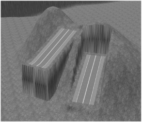
The road mesh is generated using a base spline and world terrain geometry that is covered by the road segment. This provides a relatively easy and intuitive way to lay down the road network. However, as shown in Figure 4.11.3, the road surface generated in such way follows the terrain surface exactly and may not be smooth enough.

The road surface must satisfy a number of conditions enforced by the road-grading tool. The most important characteristics controlled by this tool are road grade and road slope. A road slope is defined as a road surface tilt (the gradient perpendicular to the road), and a road grade is defined as steepness of the road (the gradient parallel to the road) [Wiest98].
The tool allows designers to set up the road grade and slope limits and automatically modify the road surface to create a realistic look and improve the routable functionality of roads. The algorithm adjusts individual or connected road segments’ tilt and steepness using height map grid cells. We describe a technique that deals with the slope and grade limits separately.
The purpose of the road slope flattening algorithm is to set to zero the slope across a road segment. The same technique can be applied to the connected road segments.
The actual road mesh modification is accomplished by a world terrain height map data modification. The advantage of this method is a smooth coupling of road surface with the surrounding terrain. The disadvantage is that the road surface geometry will become imprinted to the terrain geometry. Moving the graded road will leave a modified terrain behind, and this may lead to visual artifacts.
Alternatively, the road network surface could be managed by a separate height map, and terrain generation code should support multiple height map layers to combine the original terrain data and road network maps.
The road segment spline defines a road profile. At the first step, we divide a road segment by sub-dividers, as shown in Figure 4.11.4.
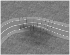
The distance between sub-dividers depends on the terrain height map resolution and the road edges’ lengths. For example, if each height map point represents a 1×1 unit in world coordinates, then the sub-divider distance could be an average value between maximum and minimum road edge lengths.
The second step is determining a height for sub-divider end points. The height of sub-divider end points should match the height of the sub-divider center point (a height at the intersection between the sub-divider and a road spline) to set zero road slope.
The third step is applying a new height to each height map point inside of a sub-quad formed by a pair of sub-dividers. Since there is no guarantee that the four points defining the sub-quad corners belong to the same plane, we need to triangulate each sub-quad and flatten the inner height map points for each triangle, as shown in Figure 4.11.5. We use the plane equation to calculate the new height of height map points inside the triangle.

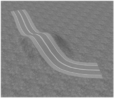
The fourth and final step is to create a smooth road surface. The results of the previous step can leave visual artifacts between road sub-quads. To fix the surface, we use a bilinear interpolation between neighboring height map points across the entire road segment. In the case of connected road segments, the bilinear interpolation should be performed across the entire road network. Figure 4.11.6 shows the result.
To limit a road segment grade, we use a modified road slope flattening technique. After the road segment subdivision, we calculate an inclination angle for each sub-quad. Then we adjust the angle by raising or lowering sub-quad dividers. The challenge here is to determine which road direction should be used for raising or lowering each end. Figure 4.11.7 shows the difference.
These algorithms were very useful during The Sims 3 development and saved a significant amount of world designers’ time by automating mesh modifications. The in-game routing system also benefited from flattened road slopes and reasonably limited road grades.
The same algorithms could also be applied to the flattening of water surfaces (such as rivers) or can be modified to achieve more complex road surfaces, such as road banking on curves. However, using such an algorithm on non-height map–based terrain meshes may require different approaches for sub-quad height calculation, surface triangle flattening, and surrounding geometry transitions.
These techniques cover a relatively complete set of road creation tasks for large environments. An abstract definition of a road as a geodesic curve may not be sufficient to deliver fully automated road creation, but it can provide a good starting point for the world designers, from which they can tweak road layout to their liking. The road-grading tool proved to be so versatile that very few (if any) manual adjustments of the meshes were required after the road was created and imprinted into the terrain.