
Krzysztof Mieloszyk, Gdansk University of Technology
Physics in real-time simulations as well as in computer games has been gaining importance. The game producers have observed that the advanced realism of the graphics is not enough to keep players content and that the virtual world created in a game should follow the rules of physics in order to behave more realistically. Until now, such realism has been mainly reflected by illustrating the interactions between the material objects. However, the phenomenon of reciprocity between such media as liquid or gas and more complex objects is also of high importance. With increasing processor power, the growing number of physics simulation methods that were initially developed purely for scientific reasons are being utilized in the entertainment market. However, simulation methods commonly used in games tend to be relatively simple in the computational sense or very focused on a specific case. An attempt to adapt them to other game variants is often impossible or requires an application of complicated parameters with values that are difficult to acquire. Hence, some more universal methods that allow for more easily modeled game physics are valuable and attractive tools for hobbyists and creators of later game extensions.
Commonly, the medium is a physical factor that in various ways affects the complete surface of the object. Hence, for the purpose of fluid dynamics simulation, every shape needs to be represented as a closed body with all its faces pointing outward and fully covering its outside surface. The inside should be looked upon as full; it must not have any empty spaces or “bubbles.” Every edge should directly contact exactly two surfaces, while the entire object mesh must fulfill the following condition:
where V= vertices, F= faces, and E= edges.
Because the preliminary interaction value is calculated on points, it is convenient to organize the mesh in a list of points in the form of coordinates and a list of triangles represented as three sequential indices of its vertices. Additionally, every triangle should have a normal vector of its surface, as well as the surface value. In some cases, depending on the computational method used, the position of the triangle center can also be useful. In this article, we will sometimes refer to vertices as points and triangle meshes as faces.
Using some physical basics of fluid mechanics (referring among others to Pascal’s Law), pressure is defined as a quotient of force F, which exercises perpendicularly to the surface sector limiting the object given, and the surface S of this sector [Bilkowski83].
The total pressure affecting the body surface in a given medium point can be represented by a sum of two components: static and dynamic pressure.
In order to define the static pressure that is needed to create buoyancy in a selected medium, we need the medium density ρ[kg/m3], gravitational field intensity g [m/s2], and the distance to the medium surface h. (In the case of air, the altitude is needed.)
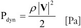
Dynamic pressure originates from the kinetic energy pressure of the medium, which results from its movement and can be determined by knowing the medium density ρ as well as the fluid velocity V [m/s] at a selected position (applicable for subsonic speed).
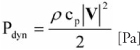
Equation (5) can be extended with a nondimensional pressure coefficient cp, whose value can be calculated as a cosine of the angle between the normal vector of the surface sector and the vector of the actual velocity in a selected point (see Figure 2.7.1). This can also be represented as a scalar product of the normal surface and the normalized velocity vector.

Figure 2.7.1. Normal vector of the surface and normal vector of velocity and the angle between them.

As an effect, we obtain a general equation for dynamic pressure exerted on a segment of the surface shown in Equation (7). The method presented in this gem solves the computation of dynamic pressure based on velocity and assumes that we use a rigid body. The use of physical models based on joints or springs is also possible.
The whole issue of calculating the pressure distribution on a mesh comes down to computing the values on the mesh vertices (or center of triangles) taking into consideration the immersion, velocity, surface area, and normal of each of the triangles that form the object. This allows us to calculate the force of the pressure that influences the physical model. Additional problems arise in the case of the object being placed in two different media simultaneously. Here the division plane separates the object faces into those faces that are totally immersed in only one medium and faces that are located in both of them. The factors requiring serious consideration are characterized in the following section.
For calculations of the static pressure affecting the object, it is necessary to define the distance h between the selected point and the medium boundary (for example, a water surface). For this, the scalar product can be applied, giving us the following Equation (8), schematically illustrated in Figure 2.7.2.

Assuming that the normal vector of the surface is pointing upward, the negative value of the obtained distance means that the point is located under the “water” surface, and the positive is above its surface. In cases when the boundary is located at the virtual world “sea level,” we know in which of the two media the point is located. To reduce the possibility of a calculation error, point Psurface (through which the surface dividing the media is crossing) should correspond to the projection of the object’s center onto this surface, in accordance with its normal vector.
Because the objects simulated in the virtual world are frequently moving, one of the most important factors needing to be improved in their dynamics is the influence of the surrounding medium. Therefore, it is required to include the velocities of each of the object mesh points (Equation (9)) as a sum of the mass center’s linear velocity Vobj and the object’s angle velocity (Figure 2.7.3). The velocity Vp obtained this way represents the global velocity for selected point P. To calculate the dynamic pressure, the local velocity vector, which is equal to the negative global point velocity, is required [Padfield96].


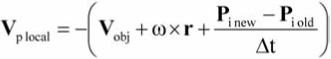
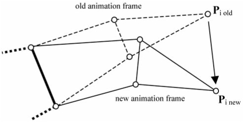
The simulated object is not always a rigid body, because some objects move by changing their body shape. A fish or a bird can be used as an example here because various body fragments of those animals move with different velocities in relation to other parts. For such objects, when calculating the point velocity, it is necessary to take the so-called morphing effect into consideration. The simplest method here is to find the change between the old and new local positions of the mesh points (see Figure 2.7.4), followed by the velocity computation, keeping the time difference Dt between the morphing animation frames in mind. As a result and an extension to Equation (9), we obtain Equation (10), which is presented below.
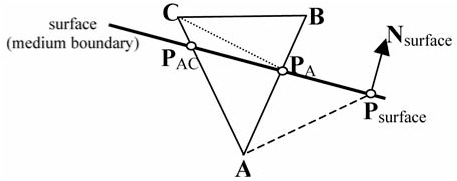
Because there is a situation in which the object triangle can be located in both media simultaneously, it is necessary to determine the borderline and find those parts that are completely submerged in only one of the media. To achieve this, the triangle should be divided into three triangles calculated by cutting points of the edges that cross the medium border. By applying Equation (11), we obtain PAB, PAC, and dividing the triangle ABC, we create a triangle A PAB PAC, located in one medium, and two arbitrary triangles located in the other medium (for example, B C PAB and C PAC PAB), as presented in Figure 2.7.5.
It is important to keep in mind that the newly created triangles must have the same normal vectors as the primary triangle. Even though each of the new triangles has the same normal, it is still necessary to recalculate the current surface area of each of those triangles. It might be very useful to apply the cross-product property, described in Equation (12), for the exemplary triangle ABC. This surface area can then be used to calculate the pressure force.


To calculate the pressure force exerted on the arbitrary triangle of the body, the pressure at each of the triangle vertices should be taken into consideration. Hence, we need to calculate the distance of each vertex from the medium surface for static pressure (Equation (6)) and the vertex local velocity, taking the angle between the velocity and the triangle surface normal into account, for dynamic pressure (Equation (7)). In the next step, the average complete pressure of the triangle vertices is calculated. However, it is useful to know that some simplifications are possible for cases when any mesh vertex has the velocity calculated from ωx r that is considerably smaller than the object linear velocity Vobj or when ω is close to zero. As a result of this, the pressure gradient distribution is almost linear, and the calculation of the complete pressure exerted on the triangle surface is reduced to obtaining the pressure in the triangle center (based on h and Vp). Thus, the pressure force is a product of a triangle normal, its surface area, and pressure (Equation (2)). For models based on a rigid body, calculation of the complete force and the torque comes down to summing the pressure forces from each surface fragment, as well summing all torques as pressure force vector cross-products and the forces at the center of the triangles.
The method for computing the static pressure presented in this gem is based solely on simple physical rules. However, the effect of dynamic pressure is one of the most complicated problems of the mechanics, for which no simple modeling method exists. The computational method used here is highly simplified and based on a heuristic parameter cp. This is sufficient for the purpose of physical simulation, which visually resembles the correct one; however, obtained values strongly diverge from the real values, resulting in too low of lift and too high of drag values. Hence, when calculating a force vector obtained from dynamic pressure, it is beneficial to introduce a correction in accordance with the velocity vector at a selected point. As in Equation (13), the factors used here are determined empirically and should be interpreted as recommended, not required. The corrected dynamic pressure force vector of the selected triangle has to be summed with the static pressure force vector occurring on its surface. The results obtained in that way approximate the results of the real object (for example, an airplane) for which the dynamic pressure is most important.
The simplified method of computing the flow around an arbitrary closed body presented here allows us to easily obtain approximate values of forces surrounding a medium. This is possible thanks to simulating some fundamental physical phenomena, such as static and dynamic pressure. Figure 2.7.6 shows screenshots from an application that interactively simulates real time using the algorithm presented here. This clearly shows a potential possibility for use in simulating the behavior of objects with fairly complicated shapes. The control here is carried out by changing the interaction between the medium and the object obtained, by morphing the shape of the object’s surface, or by moving or rotating the object elements. This allows us to create controlled planes, ships, airships, submarines, hydrofoils, seaplanes, swimming surfers, or drifting objects, as well as objects that undergo morphing, such as birds or fish. All of this is simulated based on the object mesh only.

Figure 2.7.6. Examples of applications: drifting object (top), static object (middle), morphing object (bottom). (Grayscale marks the pressure distribution in the middle and bottom images.)
The simplifications used in the algorithm bring some inaccuracies. The main problem here is the lack of consideration for the reciprocal interferential influences for each face on the final pressure values. This is a consequence of analyzing each face separately, as if it were moving in the flow consistent with its own velocity. In reality, the velocity of the flow at a given fragment of the body surface depends on the velocity over the adjacent surface fragments [Wendt96, Ferziger96]. Dependence of the value on the pressure coefficient parameter cp (as angle cosine) is a generalization. In fact, this issue would require some more specialized characteristics. Another drawback of the material presented here is that the medium viscosity has not been taken into consideration, which also adds to inaccuracies in the results. These computation versus performance tradeoffs need to be evaluated when comparing real-time methods and those that may be used in fluid dynamics engineering and design.
Implementations of the equations in this article motivated by specific examples are available on the CD-ROM.