The PASFV algorithm [Hale08] is an iterative algorithm that can be broken down into a series of simple steps. First, a set of invariants and starting conditions must be established and maintained. For our implementation of PASFV, all of the input geometry must be convex. This allows the use of the point-in-convex-object collision test [Schneider03] when determining whether a growing region has intruded into a positive space area. If the input geometry is not natively convex, it can be converted to be convex by using a triangular subdivision algorithm. While the algorithm is running, the following two conditions must be maintained to have a successful decomposition. First, at the end of every growth cycle, all the negative space regions in the world must be convex; otherwise, the collision detection tests, which are based on an assumption of convexity, will return invalid data. Second, if a region has ended a growth cycle covering an area of the level, it must continue to cover that area. If this restriction is not maintained, there will be gaps in the final decomposition.

Our algorithm begins in a state we refer to as the initial seeding state, where the world is “seeded” with a user-defined grid at specified intervals of negative space regions. These regions will grow and decompose the world. If the proposed seed placement falls within a positive space obstruction, it is discarded. Initial regions are unit squares (a unit square is a square with an edge length equal to one of the base units of the world) with four edges arranged in a counterclockwise direction from the point closest to the origin.

The initial placement of these regions in the world is such that they are axis-aligned. After being seeded in the world, each of the placed regions is iteratively provided a chance to grow. Growth is defined for a region as a chance to move each edge outward individually in the direction of each edge’s normal. The decomposition of a level may take two general cases. The first case occurs when all of the positive space regions are axis-aligned. The more advanced decomposition case occurs if there is non-axis-aligned geometry.

First, we will examine the base case or axis-aligned case for a spatial decomposition in PASFV. Growth occurs in the direction of the normal for each of the edges of a region and is a single unit in length. After an edge has advanced, we verify the new regional coverage with three collision detection tests. We want to guarantee that no points from our newly expanded region have intruded into any of the other regions or any positive space obstructions. We also want to prove that no points from other regions or obstructions would be contained within the growing region. Finally, the region will perform a self-test to ensure that the region is still convex. This final check is not necessary for the base case of the axis-aligned world and can be omitted if there are no non-axis-aligned collision objects. Assuming all tests return results showing there are no collisions or violations of convexity, the region finalizes its current shape, and the next region grows.

If a collision is detected, several things must be done to correct it. First, the growing region must return to its previous shape. At this point, since both the region and the obstruction it collided with are axis-aligned, we know the region is parallel and adjacent to the object, as shown in Figure 3.3.1(a). Stopping growth here will provide an excellent representation of free space near the collided object. Finally, we set a flag on the edge of the region where the collision occurred. This flag indicates the edge should not attempt to grow again. The iterative growth proceeds until no region is able to grow. This method of growth is sufficient to deal with axis-aligned worlds and produces results similar to traditional SFV.

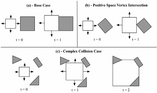
Figure 3.3.1. In this illustration we see all of the potential collision cases in PASFV. The growing negative space regions are shown as white boxes, and the direction of growth is marked with an arrow. Positive space regions are drawn in gray. In (a) we see the most basic axis-aligned collision case. Then (b) shows the collision case that occurs when a vertex of a positive space object intersects a growing negative space region. Finally, in (c) we illustrate the most complex case, where a negative space region is subdivided into a higher-order polygon to better adapt to world geometry.

The advanced case algorithm for PASFV is able to deal with a much wider variety of world environments. This case begins by building from the base case algorithm; however, because it needs to deal with non-axis-aligned positive space regions, it incorporates several new ways of dealing with potential collisions. When a collision with a positive space object occurs, one of three cases handles the collision. The first case occurs if the colliding edge of the positive space object is parallel to the edge of the growing negative space region. The particular obstruction is axis-aligned, so we revert to the base case.

The second case occurs when a single vertex of an obstruction collides with a growing edge, as shown in Figure 3.3.1(b). In this case, there is, unfortunately, nothing we can do to grow further in this direction. This occurs because unless we are willing to lose the convex property of the region or relinquish some of the area already covered by the region, doing either of these things would violate our invariants. This case reverts to the base case, and the negative space around the object will have to be covered by additional seeding passes, which are described at the end of this section.

The final, most complex, collision case occurs when a vertex of the growing region collides with a non-axis-aligned edge of a positive space obstruction, as shown in Figure 3.3.1(c). In this case, the colliding vertex must be split into a pair of new vertices and a new edge inserted between them. This increases the order of the polygon that collided with the obstruction. The directions of growth for these two newly created vertices are modified so they will follow the line equation for the edge that they collided with instead of the normal of the edge they were on.

In addition, potential expansions of these new vertices are limited to the extent of the positive space edge they collided with. In this manner, the original edges, which were adjacent to the collision point, grow outward. This outward movement expands the newly created edge, so that it is spread out along the obstruction. Limiting the growth of these vertices is important because they are creating a non-axis-aligned edge as they expand. As long as this newly generated non-axis-aligned edge is adjacent to positive space, no other region can interact with it, and we limit region-to-region collisions to the base case.

By using these three advanced case collision solutions, we are able to generate high-quality decompositions for non-axis-aligned worlds. As in the simple case with an axis-aligned world, the algorithm stops once all of the regions present in the world are unable to grow any further.

The aforementioned growth methods are not, by themselves, enough to ensure that the entirety of the world is covered by the resulting navigation mesh. In particular, the decompositions resulting from the second collision case are suboptimal. In order to deal with these issues, the second half of the PASFV algorithm comes into play. After all growth has terminated, the algorithm enters a new seeding phase. In this phase, each region places new regions (seeds) in any adjacent unclaimed free space, and then we flag the region as seeded so they will not be considered if there are any later seeding passes. If any seeds are placed, they are provided the opportunity for growth like the originally placed regions. This cycle of growth and seeding repeats until there are no new seeds placed in the world, as shown in Figure 3.3.2. At this point, the algorithm has fully decomposed the world and terminates.

Figure 3.3.2. In this illustration we see several growth and seeding cycles in the PASFV algorithm to decompose an area. The growing negative space regions are shown as white boxes, and the direction of growth is marked with an arrow. Positive space regions are drawn in gray.

The Volumetric Adaptive Space Filling Volume (VASFV) algorithm [Hale09] is a natural extension of the PASFV algorithm. Unlike PASFV, the VASFV algorithm works in native 3D and grows cubes and higher-order polyhedrons instead of quads. The initial constraint of convex input shapes is the same for both algorithms. In addition, the requirements that decomposed areas remain decomposed and that all regions always end a growth step in a convex state are still necessary.

The initial setup of VASFV is very similar to its predecessor. Both algorithms begin by seeding a grid of initial regions throughout the world. In VASFV, the grid extends upward along the Z-axis of the world as well as X-axis and Y-axis. Then, in the first of many departures from the previous algorithm, the seeds fall down in the direction of gravity until they come to rest on an object. Seeds that end in the same location are removed. This helps to prevent the formation of large, relatively useless regions that float above the level and allows the ground-based regions to grow up to the maximum allowable height. These seeds are initially spawned as unit cubes represented as regions with four faces listed in a counterclockwise order, starting with the closest to the origin followed by the bottom and top faces, respectively. At this point, the regions may grow and expand.

As with the planar version of this algorithm, there are two main cases to deal with: axis-aligned and non-axis-aligned worlds. The base case for the axis-aligned world proceeds in a manner almost identical to the planar algorithm. Each region is iteratively provided the opportunity to grow out each face one unit in the direction of the normal of each face. We then run the same three tests for error conditions as performed in the planar version of the algorithm. As a reminder, these three tests are checks to ensure that the growing region has not intersected an existing region or obstruction with one of its vertices, that no region’s or object’s vertices have intersected the newly expanded region with their vertices, and that the region is still convex. If any of these checks fail, the region will revert to its previous size and not attempt to grow again in that direction. These steps are identical to the planar case; however, the secondary algorithms required to implement them are more complex in 3D. As with the planar version of this algorithm, this base case will produce a very good decomposition of an axis-aligned world.

Like the planar version of the algorithm, the advanced growth case for dealing with collisions with non-axis-aligned geometry can be broken down into four cases (shown in Figure 3.3.3). The primary determining factor of which of the cases the algorithm will go into is determined by how many vertices are in collision and whether negative space vertices collide with positive space, or vice versa. The simplest case occurs when the growing cubic region has intersected one or more vertices of a positive space obstruction. Just like in 2D, since there is nothing that the growth algorithm can do to better approximate the free space around the object it has collided with, it returns to its previous valid shape, halting further growth in that direction.

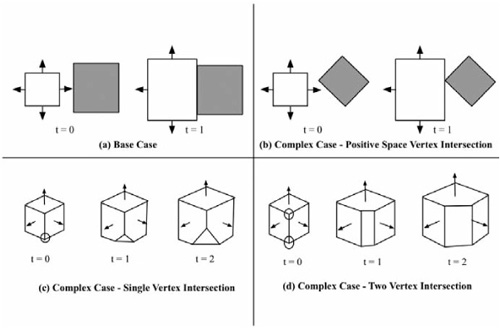
Figure 3.3.3. This illustration shows the possible collision cases for the VASFV algorithm. The growing negative space regions are shown in white. The positive space objects are shown in gray. Section (a) shows the base axis-aligned collision case from above. Section (b) shows the more complex positive space vertex collision case, again from above. Sections (c) and (d) are illustrated slightly differently. In order to clearly show how the negative space region reacts to a positive space collision, the positive space object is not drawn, and the colliding vertex is marked with a circle. Section (c) shows the single vertex collision case where a new triangular face is inserted into the negative space region. Section (d) shows the more complex two-vertex collision where a quadrilateral face is inserted into a negative space region to better approximate the object it collided with.

The next three collision cases occur when vertices from a single face of the growing negative space region intersect positive space. The first and simplest of these cases occurs when three or more vertices of a negative space region intersect the same face of a positive space object. When this happens, it means that the growing face of the negative space object is parallel to and collinear with the face of the positive space obstruction it intersected. Therefore, these two faces are both axis-aligned. We know this because three points define a plane, so by sharing these three points, both of these faces are on the same plane. This tells us that since the negative space face is axis-aligned, the positive space face we collided with must be as well. We can thus revert to the base case for this collision.

The final two collision cases require the insertion of a new face into the negative space region so that it adapts to the face of the collided object. The first case occurs when a single vertex of the region intersects an obstruction. In this case, the vertex will be subdivided into three new vertices, and a new triangular face is inserted (which has the same plane equation as the face of the object it collided with). The normal of this new face will be the inverse of the normal of the face of the intersected obstruction. These new points are restricted to prevent them from growing beyond the face of the obstruction they collided with in order to not create more non-axis-aligned geometry.

The final collision case occurs when exactly two vertices of a negative space region intersect another object. This means that a single edge of the region is in contact with the shape it collided with and that edge needs to be split. We split the edge by adding a new rectangular face to the region and by subdividing each colliding vertex into two vertices. This new face is once again created using the negation of the normal of the face it would intersect. The points involved in the collision are restricted to growing just along the collided obstruction. With the last two special collision cases, it is possible to generate navigation meshes with a degree of accuracy and fidelity to the underlying level that is not possible using previous growth-based techniques.

Like the planar version of this algorithm, VASFV also uses a seeding algorithm to ensure full coverage of a level. However, the volumetric seeding approach is slightly different from the planar version. Once each region has reached its maximum possible extents, the seeding algorithm iteratively provides each region a chance to create new seeds in adjacent negative space regions. However, instead of immediately growing the new regions, the newly placed seeds are subjected to a simulated gravity and projected downward until they hit something, and duplicate seeds that end up occupying the same space as already placed seeds are removed. At this point, the algorithm allows the newly placed seeds a chance to grow. This cycle of growth and seeding repeats until no new seeds are successfully placed, at which point the algorithm terminates.

The application of gravity to seeds might not be the most obvious approach to seeding in 3D, but it serves an important purpose in orienting region growth to better accommodate agent movement through the world. A good example of this occurs on staircases. First, consider the case where seeds do not drop due to gravity. As shown in Figure 3.3.4, a region that grows up adjacent to the bottom of the stairs will generate a single seed midway up the stairs, which will contain air space above the first several stairs and only land on one of the middle stairs. Then later seedings will result in a confusing mess of regions, none of which accurately models stair usage. Some of these regions require the agent to crawl through, while other regions require the agent to fly.

Figure 3.3.4. This figure serves to illustrate how gravity affects the seeding process for VASFV. In this figure, we see a staircase viewed from the side. Positive space regions are marked in white. Negative space regions in this illustration are marked with the light gray gradient. The upper set of four time steps shows what happens if the generated seeds are allowed to float freely and grow in midair. The lower six time steps show how the decomposition changes to better model the stair steps after the application of gravity to each generated seed.

Now consider the same staircase decomposed using a gravity-based seeding method. With gravity-assisted seeding, when a seed is generated from the initial region at the bottom of the stairs, it falls into the floor space of the first stair. The seed then grows outward to fully decompose the floor of that single stair and grows up into the airspace over the stair. In this manner, the seeds gradually climb the stairs, and each stair will become its own logical region, which makes sense given how stairs are typically traversed. This gravity-based seeding is also applicable to other methods of world space traversal, such as flight, because biasing the decomposition world in respect to the features present on the ground still makes sense.