
Udeepta Bordoloi, Benedict R. Gaster, and Marc Romankewicz, Advanced Micro Devices
Open Compute Language (OpenCL) [Munshi09] is an open standard for data-and task-parallel programming on CPUs and GPUs. It is developed by the Khronos Group, which is part of the Compute Working Group and includes members from AMD, Apple, Electronic Arts, IBM, Intel, NVIDIA, Qualcomm, and others. OpenCL is a standard to enable parallel programming on heterogeneous compute platforms. It can provide access to all the machine’s compute resources, including CPUs and GPUs.
In this gem, we give a primer on OpenCL and then introduce a set of general techniques for using it to optimize games. Two examples are used: convolution and histogram. The former highlights many of the techniques for optimizing nested loop data parallelism; the latter showcases methods for accessing memory effectively.
Convolution is a technique in the field of image processing; it calculates an output pixel as a function of its corresponding input pixel and the values of the neighboring pixels. This technique, however, is expensive to compute. Its run time is proportional to the width and height of the image. If W and H are the width and height, respectively, the run time is O(W2 H2). The highly data-parallel nature of convolution makes it an excellent candidate for leveraging OpenCL optimizations.
In game programming, histograms improve the dynamic range of rendered frames through tone mapping. Fast on-GPU histogram computation is essential, since the image data originates on the GPU. Historically, histogram computation has been difficult to do on GPU, as typical algorithms become limited by the scatter (random write-access) performance. However, with the advent of large on-chip, user-controlled memories and related atomic operations, performance can be dramatically improved.
Efficient implementations for convolution and histogram calculations broaden the set of possibilities for game developers to exploit emerging heterogeneous parallel architectures; both PCs and game consoles have many-core CPUs and GPUs. They also highlight the difficulties that must be overcome to achieve anything like peak performance.
In this gem, we discuss a step-by-step optimization toolkit for game developers using OpenCL. These optimizations can be used together or individually, but their overall effect depends on the application; there is no magic wand for an algorithm with little parallelism or a dataset so small that there is little chance to amortize the associated run-time cost.
OpenCL is based on the notion of a host API, which consists of a platform and run-time layer and a C-like language (OpenCL C) for programming compute devices; these devices can range from CPUs to GPUs and other kinds of accelerators. Figure 7.1.1 illustrates this model, with queues of commands, reading/writing data, and executing kernels for specific devices. The overall system is called a platform. There can be any number of platforms from different vendors within a particular system, but only devices within a single platform can share data within what OpenCL calls a context.
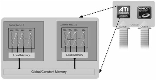
The devices are capable of running data- and task-parallel work; a kernel can be executed as a function of multidimensional domains of indices. Each element is called a work-item; the total number of indices is defined as the global work-size. The global work-size can be divided into sub-domains, called work-groups, and individual work-items within a group can communicate through global or locally shared memory. Work-items are synchronized through barrier or fence operations. Figure 7.1.1 is a representation of the host/device architecture with a single platform, consisting of a GPU and a CPU.
Given an enumeration of platforms, we choose one, select a device or devices to create a context, allocate memory, create device-specific command queues used to submit work to a specific device, and perform computations. Essentially, the platform layer is the gateway to accessing specific devices. Given these devices and a corresponding context, the application is unlikely to have to refer to the platform layer again. It is the context that drives communication with, and between, specific devices. A context generally is created from one or more devices. A context allows us to:
Create a command queue.
Create programs to run on one or more associated devices.
Create kernels within those programs.
Allocate memory buffers or images, either on the host or on the device(s). (Memory can be copied between the host and device.)
Write data to the device.
Submit the kernel (with appropriate arguments) to the command queue for execution.
Read data back to the host from the device.
The relationship between context(s), device(s), buffer(s), program(s), kernel(s), and command queue(s) is best seen by looking at sample code. The following program adds the elements of two input buffers, a and b, and stores the results in a single output buffer, o. While trivial in its application, the sample program is the foundational pattern of all OpenCL programs.
  #include <CL/cl.hpp>
  #include <iostream>
  static char kernelSourceCode[] =
  "__kernel void
"
  "hello(__global int * inA, __global int * inB, __global int * out)
"
  "{
"
  "    size_t i = get_global_id(0);
"
  "    out[i] = inA[i] + inB[i];
"
  "}
";
  int main(void) {
      int a[10] = {1,2,3,4,5,6,7,8,9,10};
      int b[10] = {1,2,3,4,5,6,7,8,9,10};
      int o[10] = {0,0,0,0,0,0,0,0,0,0};
      cl::Context context(CL_DEVICE_TYPE_ALL);
      std::vector<cl::Device> devices = context.getInfo<CL_CONTEXT_DEVICES>();
      cl::CommandQueue queue(context, devices[0]);
      cl::Program::Sources sources(1, std::make_pair(kernelSourceCode, 0));
      cl::Program program(context, sources);
      program.build(devices);
      cl::Kernel kernel(program, "hello");
      cl::Buffer inA(context,CL_MEM_READ_ONLY,10 * sizeof(int));
      cl::Buffer inB(context,CL_MEM_READ_ONLY,10 * sizeof(int));
      cl::Buffer out(context,CL_MEM_WRITE_ONLY,10 * sizeof(int));
      queue.enqueueWriteBuffer(inA,CL_TRUE,0,10 * sizeof(int),a);
      queue.enqueueWriteBuffer(inB,CL_TRUE,0,10 * sizeof(int),b);
      kernel.setArg(0,inA); kernel.setArg(1,inB); kernel.setArg(2,out);
      queue.enqueueNDRangeKernel(
      kernel, cl::NullRange, cl::NDRange(10), cl::NDRange(2)
  );
  queue.enqueueReadBuffer(out,CL_TRUE,0,10 * sizeof(int),o);
  std::cout << "{" ;
  for (int i = 0; i < 10; i++) {
       std::cout << o[i] << (i!=9 ? ", " : "") ;
  }
  std::cout << "}" << std::endl;

}
Because it is not possible to provide a full introduction to OpenCL in the limited amount of space allocated to this gem, we advise readers new to OpenCL to read through the references given at the end of the article. For example, many introductory samples are shipped with particular implementations, and readers might also like to work though a tutorial such as “hello world” [Gaster09].
Two-dimensional convolution is used to illustrate techniques that can be used to optimize OpenCL kernels.
The OpenCL C kernel for convolution is given below. It is almost a replica of a corresponding C code for convolution; the only difference is that the C code uses two for loops that iterate over the output image to initialize the variables xOut and yOut, instead of using the get_global_id call. The output image dimensions are width by height, the input image width is inWidth (equals width+filterWidth-1), and the input height equals (height+filterWidth-1).
__kernel void Convolve(__global float * input,
                      __constant float * filter, __global float * output,
                      int inWidth, int width, int height, int filterWidth)
{
    int yOut = get_global_id(1);//for (int yOut = 0; yOut < height; yOut++)
    int xOut = get_global_id(0);//for (int xOut = 0; xOut < width; xOut++)
    int xInTopLeft = xOut; int yInTopLeft = yOut;
    float sum = 0;
    for (int r = 0; r < filterWidth; r++) {
        int idxFtmp = r * filterWidth;
        int yIn = yInTopLeft + r;
        int idxIntmp = yIn * inWidth + xInTopLeft;
        for (int c = 0; c < filterWidth; c++)
            sum += filter[idxFtmp+c]*input[idxIntmp+c];
    } //for (int r = 0...
    int idxOut = yOut * width + xOut;
    output[idxOut] = sum;
}
Figure 7.1.2 shows the computation time for an output image of size 8192×8192. The test computer is an AMD Phenom X4 9950 Black Edition with 8 GB RAM. For a filter width of 2, the input image size is 8193×8193; for a filter of width 32, the input image is 8223×8223. For each pixel, the loop runs for (filterWidth)2 times. The computation time increases approximately as a function of the square of the filter width. It takes about 14.54 seconds for a 20×20 filter and 3.73 seconds for a 10×10 filter. We first consider unrolling loops to improve performance of this workload.

Having loops in the code comes at a performance cost. For example, consider a 32×32 filter. For each pixel in the output image, the statements in the innermost loop are run 32×32 = 1024 times. This cost is negligible for small filters, but it becomes significant as the filter width increases. The solution is to reduce the loop count.
The following kernel has four iterations of the innermost loop unrolled. A second loop is added to handle the remainder of iterations when filter width is not an even multiple of four.
__kernel void ConvolveUnroll(...)
{
...
for (int r = 0; r < filterWidth; r++){
...
int c = 0;
while (c <= filterWidth-4) {
sum += filter[idxFtmp+c] *input[idxIntmp+c];
sum += filter[idxFtmp+c+1]*input[idxIntmp+c+1];
sum += filter[idxFtmp+c+2]*input[idxIntmp+c+2];
sum += filter[idxFtmp+c+3]*input[idxIntmp+c+3];
c += 4;
}
for (int c1 = c; c1 < filterWidth; c1++)
sum += filter[idxFtmp+c1]*input[idxIntmp+c1];
} //for (int r = 0...
...
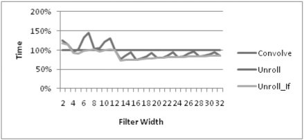
}Figure 7.1.3 shows the results of the unrolled kernel. For larger filters, unrolling helps improve speed by as much as 20 percent. The sawtooth kind of behavior that we see in the graph is due to the iterations that are left over after unrolling and is easily handled by unrolling the second inner loop (and substituting it with an if-else statement).
For the aforementioned kernels, filter widths were passed as an argument. Consider an application where the filter size is constant (for example, 5×5). In this case, the inner loop can be unrolled five times, and the loop condition can be removed.
__kernel void DefConvolve(...)
{
    ...
    for (int r = 0; r < FILTER_WIDTH; r++) {
        int idxFtmp = r * FILTER_WIDTH;
        ...
        for (int c = 0; c < FILTER_WIDTH; c++)
    ...
}
As the filter width is static, FILTER_WIDTH, it can be defined when building the OpenCL program. The following code shows how to pass in the value of the invariant.
std::string sourceStr = FileToString(kernelFileName);
cl::Program::Sources sources(1, std::make_pair(sourceStr.c_str(),
                                               sourceStr.length()));
program = cl::Program(context, sources);
char options[128];
sprintf(options, “-DFILTER_WIDTH=%d”, param.filterWidth);
program.build(devices, options);
cl::Kernel kernel = cl::Kernel(program, kernelName.c_str());
Figure 7.1.4 shows that defining the filter width as an invariant helps the DefConvolve kernel gain about 20 percent performance over the Convolve kernel, particularly for small kernel sizes.

Since the inner loop of the unrolled kernel has four products and four additions, it is possible to use one vector (SSE or GPU) packed-multiply and one packed-add to achieve the same results. But how do we use vectors in an OpenCL kernel? AMD’s OpenCL implementation will try to use “packed-arithmetic” instructions whenever it encounters a vector data type in the kernel. The following kernel body uses the vector type float4. Note the additional loop at the end to handle any remaining iterations when filter width is not an even multiple of four.
__kernel void ConvolveFloat4(...) {
    ...
    float4 sum4 = 0;
    for (int r = 0; r < filterWidth; r++) {
        ...
        int c = 0; int c4 = 0;
        while (c <= filterWidth-4) {
            float4 filter4 = vload4(c4, filter+idxFtmp);
            float4 in4     = vload4(c4, input +idxIntmp);
            sum4 += in4 * filter4;
            c += 4; c4++;
        }
        for (int c1 = c; c1 < filterWidth; c1++)
            sum4.x += filter[idxFtmp+c1]*input[idxIntmp+c1];
    } //for (int r = 0...
    int idxOut = yOut * width + xOut;
    output[idxOut] = sum4.x + sum4.y + sum4.z + sum4.w;
}
The second inner loop can be unrolled (kernel ConvolveFloat4_If), and invariants can be used for further speedups (kernels DefFloat4 and DefFloat4_If). Figure 7.1.5 shows the results for the vectorized kernel.

So far, our optimizations have focused on how to maximize ALU throughput. In the following section, we use a histogram calculation to address techniques for optimizing kernels limited by memory performance.
For simplicity, we assume that a histogram consists of 32-bit-per-pixel images with 256 32-bit bins. The algorithm parallelizes the computation over a number of workgroups, each of which uses a number of sub-histograms stored in on-chip __local memory.
When choosing the optimal number of work-items and work-groups, some constraints follow automatically from the algorithm, the device architecture, and the size of __local memory.
__local memory is shared within a single work-group. For the histogram algorithm, it is desirable to have fewer, larger work-groups. This allows many successive threads to contribute to the same __local memory area. Conversely, using more and smaller work-groups would require costly flushing of __local sub-histograms to __global memory more frequently, since the lifetime of a work-group is shorter.
To maximize the use of __local memory, the number of work-groups should be as close as possible to the number of compute units. Each compute unit typically has a dedicated block of __local memory, and using as many of them concurrently as possible is advantageous.
The actual number of compute units, typically in the tens per GPU, can be queried at run time using:
clGetDeviceInfo( ..., CL_DEVICE_MAX_COMPUTE_UNITS, ... );
A work-group should be at least as big as the basic hardware unit for scheduling. On AMD GPUs, a wavefront is a hardware unit of work-items executing concurrently on a given compute unit. OpenCL work-groups are executed as a collection of wavefronts. Wavefront size cannot be queried via OpenCL—on current high-end AMD GPUs, it is 64 work-items. Also, a total of two wavefronts can be scheduled to run on a single compute unit at a time.
This sets an absolute minimum for the total work-item number: Multiply two times the wavefront size with the number of work-groups. An integer multiple of that number is often advisable, as it will allow more flexibility for run-time scheduling—hiding memory latency, allocating register use, and so on. On the other hand, the upper limit of the number of threads is given by the maximum work-group size times the chosen number of work-groups. The maximum work-group size can be queried using:
clGetDeviceInfo( ..., CL_DEVICE_MAX_WORK_GROUP_SIZE, ... );
Within this range, fine-tuning remains an algorithm- and kernel-specific matter. Kernels can request a particular set of resources. For example, they can request the number of registers, the size of the __local buffer, and the number of instructions. These parameters influence how the kernel is scheduled on the GPU at run time. Possible tuning knobs include the number of groups, the group size, and the number of work-items. The upcoming section on optimal read patterns gives an example.
For any implementation of either a parallel or a serial histogram, very few arithmetic operations are required. This implies that the first limiting factor for histogram performance is the read bandwidth from __global memory, as the input image originates from there. Fortunately, because the histogram read is order-independent, it is possible to optimize each work-item’s read pattern to that which is best supported by the GPU or CPU.
The CPU/GPU memory subsystem and the compiler tool chain are optimized for 128-bit quantities—the common shader pixel size of four 32-bit floats. On the GPU, multiples of these quantities are advantageous to allow the memory subsystem to take advantage of the wide (typically hundreds of bits) data path to memory. Ideally, all simultaneously executing work-items read adjacent 128-bit quantities, so that these can be combined to larger quantities.
This leads to the following access pattern: Each thread reads unsigned integer quantities packed into four-wide vectors (uint4) quantities, starting at its global work-item index and continuing with a stride equal to the number of threads, until it reaches the end. For a total work-item number of NT, the resulting pattern is:
uint4 addr | 0 | 1 | 2 | 3 | ... | NT-4 | NT-3 | NT-2 | NT-1 |
Thread | 0 | 1 | 2 | 3 | ... | NT-4 | NT-3 | NT-2 | NT-1 |
uint4 addr | NT | NT+1 | NT+2 | NT+3 | ... | 2NT-4 | 2NT-3 | 2NT-2 | 2NT-1 |
Thread | 0 | 1 | 2 | 3 | ... | NT-4 | NT-3 | NT-2 | NT-1 |
As many of the work-items execute this step at the same time, it results in a large number of simultaneous, adjacent read requests, which can be combined into optimal hardware units by the memory subsystem. For example, for NT = 8192, the addresses sent to the memory subsystem result in a tightly aligned pattern:
Thread | 0 | 1 | 2 | 3 | 4 | ... | 8189 | 8190 | 8192 |
uint4 addr | 0 | 1 | 2 | 3 | 4 | ... | 8189 | 8190 | 8192 |
Note that the straightforward choice—a serial access pattern from within each work-item—results in widely dispersed concurrent accesses when issued across all active threads; this is a worst-case scenario for the GPU. Here, NI is the number of uint4 items per thread:
uint4 addr | 0 | 1 | 2 | 3 | ... | NI-4 | NI-3 | NI-2 | NI-1 |
Thread | 0 | 0 | 0 | 0 | ... | 0 | 0 | 0 | 0 |
uint4 addr | NI | NI+1 | NI+2 | NI+3 | ... | 2NI-4 | 2NI-3 | 2NI-2 | 2NI-1 |
Thread | 1 | 1 | 1 | 1 | ... | 1 | 1 | 1 | 1 |
As an example, for NT = 8192 and NI = 128, the addresses sent to the memory subsystem are widely dispersed:
Thread | 0 | 1 | 2 | 3 | 4 | 5 | 6 | 7 | ... |
uint4 addr | 0 | 128 | 256 | 320 | 512 | 640 | 768 | 896 | ... |
On the CPU, this pattern is nearly ideal, particularly when running only a few CPU work-items with large numbers of NI. Each work-item reads sequentially through its own portion of the dataset; this allows prefetching and per-core cache line reads to be most effective. As a rule of thumb, it is desirable to use per-thread column-major access on the GPU and per-thread row-major access on the CPU. Row-major and column-major access can be implemented in a single kernel through different strides—a kernel can switch at run time without cost.
Both patterns are shown in the following code example, where nItemsPerThread is the overall number of uint4 elements in the input buffer, divided by the number of threads:
__kernel void singleBinHistogram (__global uint4 *Image,
                                  __global uint *Histogram,
                                  uint nItemsPerThread )
{
    uint id = get_global_id(0);
    uint nWItems = get_global_size(0);
    uint i, idx; uint bin = 0;
    uint val = SOME_PIXEL_VAL;
#ifdef GPU_PEAK_READ_PERF
    // with stride, fast
    for( i=0, idx=get_global_id(0); i<nItemsPerThread; i++, idx+=nWItems) {
#else
    // serial, slow on GPU, fast on CPU
    for( i=0, idx=0; i<nItemsPerThread; i++, idx+=1 ) {
#endif
        if( Image[idx].x == val ) bin++;
        if( Image[idx].y == val ) bin++;
        if( Image[idx].z == val ) bin++;
        if( Image[idx].w == val ) bin++;
   }

   Histogram[id] = bin;
}
When executed with at least 8192 work-items and a work-group size of 64, this kernel reaches near hardware peak performance (on AMD GPUs), as shown in Figure 7.1.6.

On the CPU, reads and randomly indexed writes can be performed at roughly the same speed. The GPU, on the other hand, excels when massively parallel writes can be coalesced into large blocks, just as was shown for reads in the previous section. Also, the total read-modify-write latency to __global memory can be a contributor. For a straightforward parallel histogram implementation, where each thread creates a sub-histogram in __global memory, as in the following code example, scatter turns out to be a bottleneck.
__kernel void multiBinHistogram ( __global uint4 *Image,
                                  __global uint *Histogram,
                                  uint nItemsPerThread ) {
    uint id = get_global_id(0);
    uint nWItems = get_global_size(0);
    uint i, idx;

    for( i=0, idx=get_global_id(0); i<nItemsPerThread; i++, idx+=nWItems )
    {
        Histogram[ id * NBINS + Image[idx].x ]++;
        Histogram[ id * NBINS + Image[idx].y ]++;
        Histogram[ id * NBINS + Image[idx].z ]++;
        Histogram[ id * NBINS + Image[idx].w ]++;
    }
   ...
}A powerful way to address the GPU scatter bottleneck is to direct scatter into __local memory. This memory is available to all work-items in a work-group, and its lifetime is that of the group.
It is fast for the following reasons:
It typically is on-chip (cf.
clGetDeviceInfo(CL_DEVICE_LOCAL_MEM_TYPE)) and very low latency. In essence, it is a user-manageable cache.It supports a large number of concurrent data paths: one for each compute unit and more for multiple banks on each compute unit, resulting in an aggregate bandwidth up to an order of magnitude higher than
__globalmemory.It allows the use of hardware atomics, so that random access RMW cycles can be performed without having to worry about expensive, explicit synchronization between the global set of threads.
The __local memory size per work-group (and by extension, per compute unit) is given by:
clGetDeviceInfo( ..., CL_DEVICE_LOCAL_MEM_SIZE, ... );
This gives a total __local size per GPU device as CL_MAX_COMPUTE_UNITS * CL_DEVICE_LOCAL_MEM_SIZE.
A straightforward implementation for the histogram algorithm would be to simply have a sub-histogram instance per __local memory and to let all threads in that group contribute to that single instance, as shown in the following example code:
__kernel void histogramLocal( __global uint4 *Image,
                              __global uint *Histogram,
                              __local uint *subhists,
                              uint nItemsPerThread ) {
    uint id = get_global_id(0);
    uint nWItems = get_global_size(0);
    uint i, idx; uint4 temp;
    // initialize __local memory
    ...
    // scatter loop
    for( i=0, idx=tid; i<nItemsPerThread; i++, idx+=nWItems ) {
       temp = Image[idx];

       atom_inc( subhists + temp.x );
       atom_inc( subhists + temp.y );
       atom_inc( subhists + temp.z );
       atom_inc( subhists + temp.w );
    }
    barrier( CLK_LOCAL_MEM_FENCE );
    // reduce sub-histogram and write out to __global for further reduction
    ...
}
This approach performs very well for randomized input data, since the collective scatter operations from all threads are distributed over the __local banks. Unfortunately, real application images can consist of large swaths of identical pixel values—a black background, for example. The resulting simultaneous atomic read-modify-write access by many threads into a single bin quickly leads to severe contention and loss of performance.
This is where __local banks become effective as the hardware provides multiple banks that can be accessed at the same time. On AMD GPUs, addresses of adjacent 32-bit words map to adjacent banks. This pattern repeats every NB addresses, where NB is the number of available banks.
For NB=32, the __local bank layout looks like this:
uint addr | 0 | 1 | 2 | 3 | ... | 28 | 29 | 30 | 31 |
bank | 0 | 1 | 2 | 3 | ... | 28 | 29 | 30 | 31 |
uint addr | 32 | 33 | 34 | 34 | ... | 60 | 61 | 62 | 63 |
bank | 0 | 1 | 2 | 3 | ... | 28 | 29 | 30 | 31 |
The goal is to map the set of running threads to as many banks as possible. In the histogram case, an easy way to do this is to maintain NB copies for each bin and use the local work-item ID to steer simultaneous writes to the same logical bin, but into separate banks.
The resulting bins are then combined after the read-scatter phase of the kernel. The optimal number of copies for each bin can be experimentally determined, but it is less than or equal to NB. The value of NB cannot be queried via OpenCL and is obtained from the hardware spec. For recent AMD GPUs, it is 32.
#define NBANKS 32
// subhists is of size: (number of histogram bins) * NBANKS
__kernel void histogramKernel( __global uint4 *Image,
                               __global uint *Histogram,
                               __local uint *subhists,
                               uint nItemsPerWI ) {
     uint id = get_global_id(0);
     uint ltid = get_local_id(0);
     uint nWItems = get_global_size(0);

     uint i, idx; uint4 temp;

     uint4 spread = (uint4) (NBANKS, NBANKS, NBANKS, NBANKS);
     uint4 offset = (uint4)(ltid, ltid, ltid, ltid);
     offset &= (uint4)(NBANKS-1, NBANKS-1, NBANKS-1, NBANKS-1);

     // initialize __local memory
     ...
     // scatter loop
     for( i=0, idx=tid; i<nItemsPerWI; i++, idx+=nWItems ) {
        temp = Image[idx] * spread + offset;
        atom_inc( subhists + temp.x );
        atom_inc( subhists + temp.y );
        atom_inc( subhists + temp.z );
        atom_inc( subhists + temp.w );
     }
     barrier( CLK_LOCAL_MEM_FENCE );
     // reduce sub-histograms, and write out to __global for further reduction
     ...
}
By spreading out read-modify-write accesses in this manner, contention is greatly reduced, if not removed. The resulting performance gain for a test image consisting of identical pixels is an order of magnitude.
In the previous sections, a selection of techniques for optimizing OpenCL programs have been described. But how should we time changes made for performance? In general, Windows’ performance counters work well, and for more detailed profiles, tools such as AMD’s CodeAnalyst Performance Analyzer or GPU PerfStudio help. In addition to these, OpenCL provides the ability to query profiling information for specific commands executed via a command queue on a device.
By default profiling is not enabled, but it can be explicitly requested at the creation of a command queue, with the following flag:
CL_QUEUE_PROFILING_ENABLE
Alternatively, profiling can be enabled for a command queue with the following API call:
queue.setProperty(CL_QUEUE_PROFILING_ENABLE, CL_TRUE);
Generally, commands are enqueued into a queue asynchronously, and the developer must use events to keep track of a command’s status, as well as to enforce dependencies. Events provide a gateway to a command’s history: They contain information detailing when the corresponding command was placed in the queue, when it was submitted to the device, and when it started and ended execution. Access to an event’s profiling information is through the following API call:
event.getProfilingInfo<cl_profiling_info>();
Valid values of the enumeration cl_profiling_info are CL_PROFILING_COMMAND_ QUEUED, CL_PROFILING_COMMAND_SUBMIT, CL_PROFILING_COMMAND_START, CL_PROFILING_ COMMAND_END.
OpenCL is a technology for describing data- and task-parallel programs that can use all compute resources, including CPUs and GPUs. While it is straightforward to get applications to run using OpenCL, it is not always simple to get the expected performance. In this article, we have outlined a number of techniques that can be used to optimize OpenCL programs. These optimizations are not a guarantee for performance; instead, they should be seen as a toolkit to be considered when optimizing an application.