
Richard Tonge, NVIDIA Corporation, [email protected]
Ben Wyatt and Ben Nicholson, Rocksteady Studios
One of the goals of the PC version of Batman: Arkham Asylum was to improve the realism and dynamism of the game environment by adding GPU-based physics effects, including cloth, fluids, and rigid body–based destruction. With fluids, we were able to add volumetric smoke and fog, which moves around players and other characters as they progress through it. With cloth, we were able to bring to life the piles of paper littering the admin areas of Arkham Asylum. These piles appear as static triangle meshes on other platforms. For rigid body dynamics, we wanted to provide large-scale destruction—for example, to demolish large concrete walls in the outdoor areas of the game. To believably break up a large wall requires the simulation of thousands of debris pieces colliding with the high triangle count environment of Batman. To achieve this in addition to running all the gameplay physics, graphics, and other game code on the CPU at high frame rates, it was clear that the effects would have to be run on the GPU.
For GPU acceleration of cloth and fluids, we were able to use NVIDIA PhysX, which already includes CUDA implementations of those features. For rigid body simulation, NVIDIA developed a GPU rigid body engine (GRB) implementing the subset of PhysX features we needed for Batman. Using GRB, physics calculations run up to three times faster than on the CPU, enabling the large-scale destruction required. This gem describes the design and implementation of GRB and its use in Batman.
Batman made use of NVIDIA’s APEX destruction module to author and simulate destructible game objects. APEX is a layer above PhysX that allows specific effects to be authored and inserted into games easily. APEX destruction allows the artist to specify how an object breaks, with APEX doing the dirty work of creating, splitting, and destroying PhysX rigid bodies when the object is shot at, blown up, or swept away by a tornado.
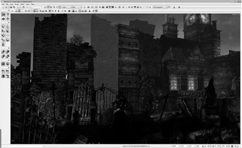
In Batman’s Scarecrow levels, large wall panels needed to be destroyed, with the debris swept up into a tornado centered on the Scarecrow. Wall panels were imported into the APEX destruction tool, where they were broken into pieces and placed into the game using Unreal Editor. With the content pipeline in place, our task was to make a GPU rigid body engine to accelerate the subset of PhysX rigid body features used by APEX destruction.
We identified the following requirements:
Performance. The system must be able to support thousands of rigid bodies colliding and interacting with the game environment in real time.
Parallelism. The system must be designed to use thousands of GPU threads to get good GPU performance and allow scaling to future GPUs.
API. The API should be similar to PhysX rigid body and support all features and API calls made by APEX destruction.
Interaction with PhysX. The game will use PhysX (CPU) rigid bodies for game-play objects (for example, Batman). GRB should support one-way interaction with PhysX bodies. (PhysX bodies should move GRBs but not vice versa.)
Shapes. GRB should support the PhysX shapes used in Batman—that is, triangle meshes, convex meshes, spheres, capsules, and boxes.
Multi-threading. The simulation should occur asynchronously to the game thread to allow unused GPU resources to be utilized whenever they occur in the frame and avoid having the game thread wait for GRB to complete.
Buffering. The game should be free to change the scene while the simulation is running without disrupting the simulation.
Streaming. Batman uses a single scene for the whole game and streams in adjacent levels as the player moves around. This means that additions to the scene have to be fast.
Authoring. It should be easy to author and tune content. Artists should be able to specify which game objects collide with GRBs and which don’t.
The static environment is represented by the original geometry used in the game—triangle meshes, convex meshes, boxes, and so on. Dynamic objects have a sphere-based representation made by voxelizing the object geometry. Color Plates 13 and 14 show how shapes in Batman are represented by voxel-generated spheres in GRB. Although spheres are used to represent the collision geometry of dynamic objects, the dynamics are still done on rigid body coordinates.
One of the most important requirements was that the algorithm be highly data parallel to allow efficient GPU implementation. Initially, the dynamics method from [Harada07] seemed like a good choice. In this method, spring and damper forces are applied at contact points to prevent penetration. The forces are integrated explicitly, which means that they can be calculated in parallel. In a sense, this method is maximally parallel, because there are as many threads as contacts.
Unfortunately, like other penalty methods, this method is hard to tune. In this method, the spring stiffness must be set high enough so that penetration is avoided for all incoming velocities. Penalizing penetration with springs injects unwanted energy into the system, so a damping parameter has to be tuned to dissipate the extra energy. Although tuning these parameters is reasonable for simple collisions—for example, between two spheres—it quickly becomes intractable for multiple simultaneous collisions each having multiple contacts. Also, because the method is an explicit method, the stiffness dictates a maximum time-step size for which the simulation is stable. [Harmon09] addresses some of these problems, but the method is far from real time.
To avoid these problems, we decided to use an implicit constraint-based method similar to that used in PhysX. In this method, instead of producing a spring and damper per contact point, the collision detection code produces a set of rules called constraints. These constraints are fed into a constraint solver, which iteratively finds a new set of velocities for the bodies. Its goal is to find velocities that won’t move the bodies into penetration (violate the constraints) in the current time step. Compared to [Harada07], implementing this method has the additional complexity of parallelizing a constraint solver. The parallelization will be described in a later section.
The following is a high-level description of the pipeline.
Transform spheres into world space using body transformation matrices.
Find sphere-sphere overlaps, producing contacts.
Find sphere-mesh overlaps, producing contacts.
Evaluate force fields, such as wind, explosions, tornados, and so on.
Update body velocities by applying force fields and gravity.
Generate constraints from contacts.
Solve constraints producing modified velocities and position corrections.
Update body positions using position corrections.
The spheres are rigidly attached to the rigid body reference frame. For this reason, in each frame the spheres have to be transformed from their local frame to world space. For a particle with position r belonging to a rigid body with transformation matrix M, we calculate the world space position as follows:
rworld = Mr
The dynamic objects are represented by grids of spheres, so we use sphere-sphere tests to determine the points of contact between them. We use the same size spheres for all the dynamic objects in the scene, so the sphere radius is a global parameter σ. A pair of spheres separated by vector rij are overlapping if |rij| ≤2σ. In this case, the contact normal nc, position pc, and separation φc are defined as follows.
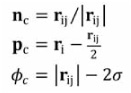
In the case, where the two spheres are in almost the same position (|rij| ≤ ε, where ε is a small positive number), we use an arbitrary contact normal nc = (1,0,0). Note that when the spheres are penetrating, the “separation” is negative.
The static environment is mainly composed of non-convex triangle meshes, so we also have to test for sphere-triangle contact. For each sphere and potentially colliding triangle, we first need to check whether the center of the sphere is already behind the triangle. Ignoring contact in this case helps avoid the situation where some of a body’s spheres are trapped on one side of a triangle and some on the other, and it also simplifies the computation of the separation. Given sphere center ps, triangle vertices (v0, v1, v2), and triangle normal nt, the sphere center is behind the triangle if:
nt.ps < nt.v0
If a sphere and triangle survive this test, then we next need to calculate world coordinates pt of the closest point on the triangle to the center of the sphere ps. For details on how to do this, see [Ericson05]. We generate a contact for a sphere and triangle if |ps – pt| ≤ σ. The contact normal, position, and separation are given by the following:
nc = (ps – pt)/|ps – pt|
pc = pt
φc = |ps – pt| – σ
In the case that the sphere center is on the triangle |ps – pt| ≤ ε, we set the contact normal nc to the triangle normal instead.
We use a uniform grid data structure to avoid having to test every sphere against every triangle in the mesh. This is described later in this gem.
Force fields are used in Batman to blow around debris and implement tornado effects. GRB supports the same interface as PhysX for specifying and evaluating force fields. See [Nvidia08] for more details.
For a body with velocity v, we step the acceleration due to force fields af and gravity ag through time step h to get the unconstrained velocity v*. We also apply a global damping parameter η.
v* = (1 – ηh)[v + h(af + ag)]
Each body’s inertia matrix I is calculated in its local frame, so we need to transform it to the world frame as follows:
where R is the orientation matrix of the body.
For each contact, the constraint solver needs a coordinate frame [b0 b1 b2] in which to apply the constraint forces. We’ll refer to these three vectors as constraint directions. The X-axis is aligned with the contact normal b0 = nc, and the other two axes are arbitrarily chosen orthogonal axes in which the friction forces will be applied.
Consider a contact with position pc, normal nc, and separation φc. Let the position of the contact relative to the center of masses of body a and body b be ra and rb, their final (constrained) velocities be ![]() and
and ![]() , their inertia be Ia and Ib, and their masses be ma and mb.
, their inertia be Ia and Ib, and their masses be ma and mb.
Each non-penetration constraint has the following form, known as the velocity Signorini condition:

Here, v0 is the component of relative velocity of the two bodies at the contact point along the contact normal, and f0 is the magnitude of the impulse calculated by the constraint solver to satisfy the constraint. The condition ensures that the bodies are either separating or resting. Additionally, if the bodies are separating, then the solver must not apply any impulse; and if the bodies are resting, then the solver must apply a non-adhesive impulse. The calculation of the friction impulses will be described later.
The constraint solver solves each constraint independently. To do this, it needs to calculate ![]() , the magnitude of the impulse to apply along direction bj needed to zero the relative velocity along that direction, given initial relative velocity vj. The constant a is the reciprocal of the effective mass and is precomputed as follows:
, the magnitude of the impulse to apply along direction bj needed to zero the relative velocity along that direction, given initial relative velocity vj. The constant a is the reciprocal of the effective mass and is precomputed as follows:
The task of the solver is as follows: Given a set of bodies with unconstrained velocities v* and a set of constraints, find impulses to apply to the bodies such that the resulting velocities will (approximately) satisfy the constraints. As with most game physics engines, GRB uses an iterative projected Gauss-Seidel solver. Given an unlimited number of iterations, the constraints will be solved exactly. In Batman, we terminate after four iterations, so although the velocities may slightly violate the constraints, we can bound the amount of time the solver will take.
Let the number of constraints be m. If friction is used, then m is the number of contacts multiplied by three. In this section, we’ll assume that the constraint directions and all the other constraint parameters are concatenated into arrays of length m. The solver iterates over the constraints, solving each in isolation.
Zero f, the impulse accumulator for each constraint
For each iteration
For i = 0 to m
Calculate the impulse required to prevent relative motion along constraint direction i
Clamp the accumulated impulse to satisfy the Signorini or friction constraint
Add impulse to impulse accumulator
Apply impulse to update the velocities of the constrained bodies
Given ![]() and
and ![]() , the linear and angular velocities of the two bodies constrained by constraint i, and ra and rb, the position of the contact in the frames of body a and body b, the relative velocity along the constraint direction bi is given by the following:
, the linear and angular velocities of the two bodies constrained by constraint i, and ra and rb, the position of the contact in the frames of body a and body b, the relative velocity along the constraint direction bi is given by the following:
In other words, vrel is the velocity of the contact point on body a minus the velocity of the contact point on body b projected onto the direction bi. We can now multiply by the inverse effective mass ai to get fd, the additional impulse required to satisfy the constraint in isolation:
fd = aivrel
Constraint i is either a non-penetration constraint or a friction constraint. For non-penetration constraints, we clamp to prevent adhesion as follows:
fnew = max(0,fi + fd)
For friction constraints, we approximate the Coulomb friction cone with a pyramid aligned to the friction constraint directions. This allows us to calculate the friction impulses separately. For a friction constraint with friction coefficient μ, we look up fj, the impulse applied at the corresponding non-penetration constraint, and then clamp to the friction pyramid as follows:
fnew = max( –μfj, min(fi + fd, μfj))

The solver calculates a new velocity for each body. To apply velocity (vlin, vang) to a body with position p, orientation quaternion q, and time step h, we use the following:
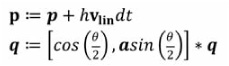
where a = vang/|vang| and θ = |hvang|.
Amdahl’s law dictates that if you parallelize less than 100 percent of your code, your speedup will be at best the reciprocal of the proportion not parallelized. For example, if 80 percent of the code is parallelized, the speedup will be no more than 5×, even though the GPU might be significantly more than five times faster than the CPU. So our initial aim was to port all stages of the GRB pipeline to the GPU. In the end, we ported all pipeline stages except for force field calculation to the GPU. The reason that we didn’t port force field calculation is that the PhysX API allows the user to write custom force evaluation kernels in C. Linking artist-generated kernels into the GRB CUDA code was not supported with the available tool chain. An advantage to running almost all of the pipeline on the GPU is that most of the data can be kept in the GPU’s memory. This is an advantage because data transfer between CPU memory and GPU memory introduces latency and unnecessary synchronization with the CPU.
The pipeline stages can be divided into those that are easily parallelized and those that are not. The stages in the first category are transform particles, find sphere-sphere contacts, find sphere-mesh contacts, update velocities, generate constraints, and update body positions. For example, in transform particles, each GPU thread is assigned a single particle. The calculation of each particle is independent, and as there are typically more than 10,000 particles in Batman, the GPU is well utilized. Similarly, each thread is assigned one particle in the collision detection stages. In the sphere-sphere stage, each thread is responsible for finding nearby particles; and in the sphere-triangle stage, each thread looks at nearby triangles. Again, each thread can do this without synchronizing with any other. In order to concatenate the contacts produced by each thread, we allocate memory for a fixed number of contacts per thread. We used four contacts per sphere in Batman. Once this fixed number of contacts has been generated, further contacts are discarded. Discarding contacts could result in unwanted penetration, but in Batman this is rarely visible. Another way to do this would be to use a scan (prefix sum) operation [Harris07] to allocate space for the contacts. However, this requires running the collision kernels twice—once to calculate the number of contacts and again to fill in the contact data. For the easily parallelized stages, the CUDA port was very quick. In most cases it was as simple as removing an outer for loop, adding the__device__ keyword, and compiling the body of the for loop with the CUDA compiler. Most of the loop bodies compiled with little or no changes.
The only pipeline stage that is not easily parallelized is the constraint solver, and that will be discussed in one of the following sections.
Voxelization is the conversion of an object into a volume representation, stored in a three-dimensional array of voxels. A voxel is the three-dimensional equivalent of a pixel, representing a small cubical volume. Since GRB represents objects as a collection of spheres, we use voxelization to generate an approximate sphere representation of the convex objects generated by APEX destruction. Each covered voxel generates a single sphere.
The voxelizer isn’t strictly part of the pipeline because it is only run when dynamic objects are first loaded. However, Batman levels are streamed, so object loading has to be as fast as possible. For this reason we decided to use a GPU voxelizer.
Initially, we implemented an OpenGL voxelizer, similar to that described in [Karabassi99]. However, this required creating a separate OpenGL context, and there was significant overhead in transferring data between OpenGL and CUDA, so we decided to write a CUDA implementation instead.
Since the shapes generated by APEX destruction were all convex meshes, this was considerably simpler than writing a general-purpose triangle mesh voxelizer. The basic algorithm used was to convert each triangle in the convex mesh into plane equation form. This way, it is simple to determine the distance of a point from any plane by performing a simple dot product. The plane data is sent to the GPU using CUDA constant memory. We then launch a kernel with one thread per voxel. Each thread loops over all the planes, calculating the distance to the plane and keeping track of the minimum distance and sign. If the point is inside all the planes, then we know it is inside the object. By discarding points more than a maximum distance away from the nearest plane, we can modify the thickness of the voxelized skin of the object.
Although this algorithm was efficient for large volumes, for GRB we typically needed only a coarse voxelization (perhaps only 83 voxels), which didn’t generate enough threads to fill the GPU. For this reason, we developed a batched voxelizer that voxelized a whole collection of convex shapes in a single kernel invocation.
One issue was that the original voxelizer would sometimes generate overlapping spheres for the initially tightly packed groups of convexes generated by APEX destruction, causing the objects to fly away prematurely. This was due to performing the voxelization in the local space of the convex object. By modifying the voxelization to be performed in world space, we ensured that the spheres generated by voxelization fitted together exactly with no overlaps.
To avoid having to test each sphere for collision against every other sphere and each sphere against every triangle in each frame, we use a spatial data structure to cull out all but nearby spheres and triangles. Because the spheres are all the same size, we use a uniform grid whose cell size is set to the sphere diameter. So for each sphere, we can find potentially overlapping spheres by querying only the 33 cells surrounding it. The triangles are also put into a uniform grid, but a separate grid is used to allow the cell size to be tuned separately. When the triangle mesh is loaded, a voxelization process is used to identify which cells the triangle passes through. Each intersection cell is given a pointer to the triangle. In Batman, triangle meshes are streamed in as the user progresses through the levels. Initially, we updated the triangle grid incrementally each time a new mesh was loaded, but we found out that regenerating the whole grid from scratch at each mesh load was more efficient. As the spheres are used to represent moving objects, the sphere grid has to be rebuilt each frame. Like [LeGrand07, Green07] we use a fast radix sort [Satish09] to do this. The grid size used for both grids is 643. A simple modulo 64 hash function is used so that the world can be bigger than 643 cells.
Unlike the other stages, the projected Gauss Seidel solver isn’t easy to parallelize. The reason for this is that each constraint reads and writes the velocities of two bodies, and each body can be affected by more than one constraint. For example, consider a stack of three spheres resting on the ground. Each body is affected by two constraints, except for the top body. If the constraints were executed in parallel by separate threads, then each body (except the top body) would be overwritten by two threads. The final value of the velocity of each body would depend on the exact order in which the constraints accessed the body, and the effect of one constraint would not be taken into account in the calculation of the other.
To get around this problem, the solver has two phases, both of which run on the GPU. The first divides the constraint list into batches of constraints that can be executed in parallel. In each batch, all bodies are modified by just one constraint. The second executes the batches in sequence, using one thread for each constraint in each batch.
We make the assumption that any system can be solved in 32 or fewer batches. The goal is that each body be modified only once in each batch and that the number of batches used be minimal. Each body is given an unsigned integer called a batch bitmap. Bit i set means that the body is modified in batch i.
Initially, all the batch bitmaps are set to zero. In the first phase, each constraint is processed by a thread in parallel. Each thread calculates the logical or (disjunction) of the batch bitmaps of its two bodies. If a bit in the result is zero, then it means that batch doesn’t modify either body, so the constraint can be processed in this batch. So, the thread finds the first zero bit in the result and attempts to atomically set it in the two bodies. If the atomic set fails (because another thread has allocated the body to the batch in the meantime), then it starts again to find a new bit that is not set for both bodies. If all the bits are set in the disjunction of the two bitmaps, then more than 32 batches are required, and the constraint is discarded.
To test the speedup of GRB, we ran the second Scarecrow level from Batman with and without GRB. When the level is run without GRB, both the gameplay and destruction rigid bodies are run on the CPU, and when the level is run with GRB, the game-play bodies are simulated using PhysX on the CPU, but the 1,600 debris chunks are simulated on the GPU using GRB. The following timings are for the 1,600 debris chunks in both cases. In both cases, the debris rigid bodies collide with each other, the gameplay rigid bodies, and the tens of thousands of triangles that make up the static environment. Because force fields are not simulated on the GPU in either PhysX or GRB, the force field calculation is excluded in both cases.
The test was run for the first 900 frames starting at the second-to-last checkpoint of the level, where a large concrete wall is destroyed and carried away by a force field. The timings are from a representative frame captured after all the chunks have been loosened from the wall. Because the timings are of the physics pipeline only, they don’t contain graphics processing time or any other game code. The timings were taken on an Intel Core 2 Quad running at 2.66 GHz with the graphics running on a GTX260 and the physics running on a second GTX260.
GRB physics frame time (1,600 bodies) | 16.5ms |
PhysX physics frame time (1,600 bodies) | 49.5ms |
Speedup | 3.0x |
In a real game, GRB running on a GPU can achieve a threefold performance increase over PhysX running on a CPU.
GRB was written by Richard Tonge, Simon Green, Steve Borho, Lihua Zhang, and Bryan Galdrikian. We’d like to thank Adam Moravanszky, Pierre Terdiman, Dilip Sequeira, Mark Harris, and all the other people who indirectly contributed to GRB. The GRB Batman destruction content was designed by Dane Johnston and Johnny Costello, and the code was integrated into the game by James Dolan, David Sullins, and Steve Borho.