
In a compelling virtual world, virtual humans play an important role in improving the illusion of life and interacting with the user in a natural way. In particular, face motion is crucial to represent a talking person and convey emotive states. In a modern video game, approximately 5 to 10 percent of the frame cycle is devoted to the animation and rendering of virtual characters, including face, body, hair, cloth, and interaction with the surrounding virtual environment and with the final user. Facial blend shapes are commonly adopted in the industry to efficiently animate virtual faces. Each blend shape represents a key pose of the face while performing an action (for example, a smiling face or raised eyebrows). By interpolating the blend shapes with each other, as depicted in Figure 2.1.1, the artist can achieve a great number of facial expressions in real time at a negligible computational cost.

However, creation of the facial blend shapes is a difficult and time-consuming task, and, more likely than not, it is still heavily dependant on the manual work of talented artists.
In this gem, I share principles and ideas for a tool that assists the artist in authoring humanoid facial blend shapes. It is based on a physical simulation of the human head, which is able to mimic the dynamic behavior of the skull, passive tissues, muscles, and skin. The idea is to let the artist design blend shapes by simply adjusting the contraction of the virtual muscles and rotating the bony jaw. The anatomical simulation is fast enough to feed back the results in real time, allowing the artist to tune the anatomical parameters interactively.
Our objective is to build a virtual model of the human head that simulates its anatomy and can be adapted to simulate the dynamics of different facial meshes. The artist models a static face mesh, and then the anatomical simulation is used to generate its blend shapes. The goal of the simulation is to create shapes that generate realistic motion. The exact accuracy of the individual muscles in a real anatomical model is not the goal.
The anatomical elements are simple yet expressive and able to capture the dynamics of a real head. The anatomical simulation must also be fast enough to be interactive (in other words, run at least at 30 fps) to allow the artist to quickly sketch, prototype, tune, and, where needed, discard facial poses.
The basic anatomical element is the skull. The anatomical model is not bound to the polygonal resolution or to the shape of the skull mesh; we require only that the skull mesh has a movable jaw. On top of the skull, the artist may design several layers of muscles and passive tissue (such as the fat under the cheeks), the so-called muscle map. The skull and the muscle map form the musculoskeletal structure that can be saved and reused for different faces. The musculoskeletal structure is morphed to fit the shape of the target face. Then, the face is bound to the muscles and to the skull, and thus it is animated through a simple and efficient numerical integration scheme.
The anatomical model is composed of different parts, most of which are deformable bodies, such as muscles, fat, and the skin. The dynamics algorithm must be stable enough to allow interaction among these parts, it must be computationally cheap to carry out the computation at an interactive rate, and it must be controllable to allow precise tuning of the muscles’ contractions. To meet these requirements, we will use Position Based Dynamics (PBD), a method introduced in [Müller06] and recently embedded in the PhysX and Bullet engines. A less formal (although limited) description was introduced in [Jakobsen03] and employed in the popular game Hitman: Codename 47.
For an easy-to-understand and complete formulation of PBD, as well as other useful knowledge about physics-based animation, you can review the publicly available SIGGRAPH course [Müller08]. In this gem, I describe PBD from an implementation point of view and focus on the aspects needed for the anatomical simulation.
In most of the numerical methods used in games, the position of particles is computed starting from the forces that are applied to the physical system. For each integration step at a given time, we obtain velocities by integrating forces, and eventually we obtain the particle’s position by integrating velocities. This means that, in general, we can only influence a particle’s position through forces.
PBD works in a different way. It is based on a simple yet effective concept: The current position of particles can be directly set according to a customizable set of geometrical constraints ![]() , where
, where ![]() is the set of particles involved in the simulation. Because the constraints could cause the resulting position to change slightly, the velocity must be recalculated using the new position and the position at the previous time step. As the position is computed, the velocity is adjusted according to the current position and the position at the previous time step. The integration steps are:
is the set of particles involved in the simulation. Because the constraints could cause the resulting position to change slightly, the velocity must be recalculated using the new position and the position at the previous time step. As the position is computed, the velocity is adjusted according to the current position and the position at the previous time step. The integration steps are:
(1) for each particle i do ![]()
(2) for each particle i do ![]()
(3) loop nbIterations times
(4) solve ![]()
(5) for each particle i
(6) ![]()
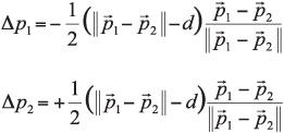
For example, let us consider the simple case of two particles traveling in the space, which must stick to a fixed distance d from each other. In this case, there is only one constraint C, which is:
Assuming a particle mass m = 1kg, Step (3) in the Algorithm 1 is solved by:
In this example, if a force is applied to ![]() , it will gain acceleration in the direction of the force, and it will move. Then, both
, it will gain acceleration in the direction of the force, and it will move. Then, both ![]() and
and ![]() will be displaced in Step (3) in order to maintain the given distance d.
will be displaced in Step (3) in order to maintain the given distance d.
Given ![]() , finding the change in position Δpi for each particle is not difficult; however, it requires some notions of vectorial calculus, which are outside the scope of this gem. The process is explained in [Müller06, Müller08] and partly extended in [Müller08b].
, finding the change in position Δpi for each particle is not difficult; however, it requires some notions of vectorial calculus, which are outside the scope of this gem. The process is explained in [Müller06, Müller08] and partly extended in [Müller08b].
Steps (3) and (4) solve the set of constraints in an iterative way. That is, each constraint is solved separately, one after the other. When the last constraint is solved, the iteration starts again from the first one, and the loop is repeated nbIterations times, eventually converging to a solution. Then, the velocity is accommodated in order to compensate the change in position Δpi. In general, using a high value for nbIterations improves the precision of the solution and the stiffness of the system, but it slows the computation. Furthermore, an exact solution is not always guaranteed because the solution of a constraint may violate another constraint.
This issue is partly solved by simply multiplying the change in position Δpi by a scalar constant K∊[0,..,1], the so-called constraint stiffness. For example, choosing k< for a distance constraint leads to a dynamics behavior similar to the one of a soft spring. Using soft constraints leads to soft dynamics and improves drastically the probability of finding an acceptable (and approximated) solution for the constraint set. For example, think about two rigid spheres that must be accommodated inside a cube with a diagonal length smaller than the sum of the diameters of the two spheres: The spheres simply will not fit. However, if the spheres were soft enough, they would change shape and eventually find a steady configuration to fit in the cube. This is exactly how soft constraints work: If they are soft enough, they will adapt and converge toward a steady state.
In my experiments, I used a time step of 16.6 ms and found that one iteration is enough in most of the cases to solve the set of constraints. Rarely did I use more iterations, and never beyond four.
Similar to the distance constraint, other constraints can be formulated considering further geometric entities, such as areas, angles, or volumes. The set of constraints defined over the particles defines the dynamics of a deformable body represented by the triangulated mesh. I provide the source code for the distance, bending, triangular area, and volume constraints on the companion CD-ROM. You are encouraged to experiment with PBD and build deformable bodies following the examples in the source code.
PBD has several advantages:
The overshooting problem typical of force-driven techniques, such as mass-spring networks, is avoided.
You can control exactly the position of a subset of particles by applying proper constraints; thus, the remaining particles will displace accordingly.
PBD scales up very well with spatial dimensions because the constraint stiffness parameter is an adimensional number, without unit of measure.
We begin the process of building our virtual head by building up the low-level pieces that make up the foundation of the physical motion. To do this, we take an anatomical approach.
The skull is the basis upon which the entire computational model of the face is built. It is represented by a triangulated mesh chosen by the artist. Figure 2.1.2 illustrates an example of the mesh used in our prototype. The skull mesh is divided in two parts: the fixed upper skull and the movable mandible. The latter will move by applying the rigid transformation depicted in Figure 2.1.2.
In our model, muscles are represented by rectangular parallelepipeds, which are deformed to match the shape of the facial muscles. To define the shape of the muscles, we draw a closed contour directly on the skull surface and the already-made muscles. Figure 2.1.3 shows an example of the definition of the initial shape of a muscle in rest state. The closed contour is defined upon underlying anatomical structures—in this case, the skull. Then, a hexahedral mesh M is morphed to fit the contour. M is passively deformed as the skull moves.

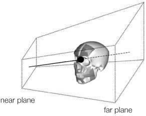
The closed contour is drawn through a simple ray-casting algorithm. The position of the pointing device (I used a mouse) is projected into the 3D scene, and a ray is cast from the near plane of the frustum to the far plane, as shown in Figure 2.1.4.
The intersection points form the basis of the muscle geometry, the so-called action lines.
An action line is a piecewise linear curve lying on at least one mesh. The purpose of the action lines is twofold: (1) They define the bottom contour of the muscle geometry during the simulation, and (2) they provide a mechanism to control the active contraction of the muscle itself. A surface point is a point sp in S, where S is the surface represented by the mesh. A surface point sp is uniquely described by the homogeneous barycentric coordinates (t1, t2, t3) with respect to the vertices A1A2A3 of the triangular facet to which it belongs, as shown in Figure 2.1.5.

Figure 2.1.5. (a) A surface point sp in A1A2A3 is defined by the homogeneous barycentric coordinates (t1, t2, t3) with respect to the triangle vertices. (b) When the triangle deforms, the triple (t1, t2, t3) does not change, and sp is updated to sp’.
The relevant attributes of a surface point are position and normal; both of them are obtained through the linear combination of the barycentric coordinates with the corresponding attributes of the triangle vertices. When the latter displace due to a deformation of the triangle, the new position and normal of sp are updated and use the new attributes of the vertices (Figure 2.1.5 (b)). Each linear segment of the action line is defined by two surface points; thus, an action line is completely described by the ordered list of its surface points. Note that each single surface point may belong to a different surface S. So, for example, an action line may start on a surface, continue on another surface, and finish on a third surface. When the underlying surfaces deform, the surface points displace, and the action line deforms accordingly.
Starting from a triangulated, rectangular parallelepiped (or hexahedron), each vertex is considered as a particle with mass m = 1; particles are connected with each other to form a network of distance constraints, as shown in Figure 2.1.6.

These constraints replicate some aspects of the dynamic behavior of a real face muscle, in particular resistance to in-plane compression, shearing, and tension stresses. Note that distance constraints are placed over the surface of the hexahedron, not internally. For completing the muscle model, we add bending constraints among the triangular faces of the mesh to conserve superficial tension. We also add a further volume constraint over all the particles, which makes the muscle thicker due to compression and thinner due to elongation.
Using the interactive editor to sketch the shape of the soft tissues over the skull, we define the structure made up of intertwined muscles, cartilage, and facial tissue, mostly fat. The muscles are organized in layers. Each layer influences the deformation of the layers on top of it, but not those underlying it. See Figure 2.1.7.

The muscle map comprises 25 linear muscles and one circular muscle. This map does not represent the real muscular structure of the human head; this is due to the simulated muscle model, which has simplified dynamics compared to the real musculoskeletal system. However, even though there may be not a one-to-one mapping with the muscle map in a real head, this virtual muscle map has been devised to mimic all the main expressive functionalities of the real one.
For instance, on the forehead area of a real head, there is a single large, flat sheet muscle, the frontalis belly, which causes almost all the motion of the eyebrows. In the virtual model, this has been represented by two separate groups of muscles, each one on a separate side of the forehead. Each group is formed by a flat linear muscle (the frontalis) and on top of it two additional muscles (named, for convenience, frontalis inner and frontalis outer). On top of them, there is the corrugator, which ends on the nasal region of the skull. Combining these muscles, the dynamics of the real frontalis belly are reproduced with a satisfying degree of visual realism, even though the single linear muscle models have simple dynamics compared to the corresponding real ones.
Each simulated muscle is linked to the underlying structures through position constraints following the position of surface points. Thus, when an anatomical structure deforms, the entire set of surface points lying on it moves as well, which in turn influences the motion of the above linked structures. For instance, when the jaw, which is part of the deepest layer, rotates, all the deformable tissues that totally or partially lie on it will be deformed as well, and so on, in a sort of chain reaction that eventually arrives at the skin.
Active contraction of a muscle is achieved by simply moving the surface points along the action lines. Given that the bottom surface of the muscles is anchored to the surface points through position constraints, when the latter move, the muscle contracts or elongates, depending on the direction of motion of the surface points.

Once the skull and the muscle map are ready, they can be morphed to fit inside the target facial mesh, which represents the external skin. The morphing is done through an interpolation function, which relies on the so-called Radial Basis Functions [Fang96]. We define two sets of 3D points, P and Q. P is a set of points defined over the surface of the skull and the muscles, and Q is a set of points defined over the skin mesh. Each point of P corresponds to one, and only one, point of Q. The position of the points in P and Q are illustrated in Figure 2.1.9 (a) and must be manually picked by the artist. These positions have been proven to be effective for describing the shape of the skull and of the human face in the context of image-based coding [Pandzic and Forchheimer02]. Given P and Q, we find the interpolation function G(p), which transforms a point pi in P and a point qi in Q. Once G(p) is defined, we apply it to all the vertices of the skull and muscle meshes, fitting them in the target mesh.

Figure 2.1.9. (a) The set of points P and Q picked on the skull and on the face mesh, respectively. (b) The outcome of the morphing technique.
Finding the interpolation function G(p) requires solving a system of linear independent equations. For each couple 〈pi,qi〉, where pi is in P and qi is the corresponding point in Q, we set an equation like:
Where n is the number of points in each set, di is the distance of pi from pj, ri is a positive number that controls the “stiffness” of the morphing, and hi is the unknown.
Solving the system leads to the values of hi, i = 1, .., n, and thus G(p):
This particular form of Radial Basis Functions is demonstrated to always have a solution, it is computationally cheap, and it is particularly effective when the number of points in P and Q is scarce. Figure 2.1.9 (b) shows an example of fitting the skull into a target skin mesh.
Skin is modeled as a deformable body; its properties are defined by geometrical constraints in a similar way to the muscles. The skin is built starting from the target face mesh provided in input. Each vertex in the mesh is handled as a particle with a mass, which is set to 1.0. After the skull and the muscle map are fitted onto the skin mesh, further constraints are defined to bind the skin to the underlying musculoskeletal structure. For each particle p in the skin mesh, a ray is cast along the normal that is toward the outer direction. In fact, after the fitting, portions of some muscles may stay outside the skin. By projecting in the outer direction, the skin vertices are first bound to these muscles. If no intersection is found, then another ray is cast in the opposite direction of the normal, toward the inner part of the head. The ray is tested against the muscles from the most superficial to the deepest one. If the ray does not intersect any muscle, then the skull is tested. The normal of the skin particle is created by averaging the normals of the star of faces to which the particle belongs.
If an intersection is found, then it is defined as a surface point sp on the intersected triangular face in the position where the ray intersects the face. A particle q is added to the system, and it is bound through a position constraint to sp. A stretching constraint is placed among the particles p and q. When the skull and the muscles move, the position of the surface points will change accordingly. The set of added particle q is updated as well because it is bound to the surface points through the corresponding position constraint and will displace the skin particles, whose final motion will depend also on the other involved constraints.
Although not very accurate from the point of view of biomechanics, the presented anatomical model is able to simulate convincing facial poses, including macro-wrinkles, which can be used as blend shapes, as shown in Color Plate 7. The model is stable, robust, and controllable, which is critical in interactive tools for producing video game content. The anatomical model is adaptive enough to animate directly the face mesh provided by the artist, thus it does not lead to the artifacts associated with motion retargeting. It does not require expensive hardware, and it may run on a consumer-class PC while still providing interactive feedback to the artist.