This section provides the general mathematics and physics background for both the linear and the quadratic drag models.

Three-Dimensional Physics

The forces for the linear model are:

And the forces for the quadratic model are given by:

where is the velocity squared, and is the unit vector that points in the direction of the velocity.

The first term of both equations is the force due to gravity, and in my representation down is the negative z direction. The direction of gravity depends on your coordinate system. The second term of both equations is the drag term. I chose the alpha and beta as different labels for the drag coefficient in order to keep it clear which version of air resistance I am referencing. For both models, if this value is big, there is a lot of fluid resistance, and if it is small, there is little fluid resistance. This parameter should always have positive value and does not actually need to remain constant. It can change if an object changes shape or angle from the direction of the fluid motion. A sail in the wind does not have a constant value, but changes depending on how taut the sail is and how perpendicular it is relative to the wind, among other factors. The velocity in these equations is the velocity of the object in the fluid, so if there is wind, then it would be the velocity of the object minus the velocity of the wind.

The linear equation is solvable in a complete analytical closed-form solution. Since the quadratic mixes all of the components of the velocity vector together, it is not solvable in a closed form, but we can solve it numerically. In addition, the quadratic drag model has the advantage of being a better approximation of realistic air and fluid resistance. Interestingly, both are exactly solvable when considered as one-dimensional problems. This will be discussed in more detail later in this gem.

Conversion from Three-Dimensional Physics to One-Dimensional Physics

To convert the drag problem from three dimensions into one dimension, we need to break the object’s motion into two components: motion along the velocity (one dimension) and motion perpendicular to the current velocity (two dimensions). The drag force only acts along the current direction of velocity; thus, we can treat it as a one-dimensional problem.

The unit vector in the direction of the velocity is given by , or if the velocity is zero it is valid to set . Setting the normal to zero works because if the object is not moving, there will be no fluid resistance. The components of the forces along the direction of motion and perpendicular to the direction of motion are shown in Figure 2.6.1. We can update the velocity along the current direction of motion as well as perpendicular to it once it is decomposed this way.

Figure 2.6.1. Breaking three-dimensional space into components along the direction of motion and perpendicular to the current direction of motion.

One-Dimensional Solutions

For a one-dimensional solution, we start from the one-dimensional version of Newton’s Second Law, F = MA, and from the definition of acceleration, a = dv/dt. If the force is a function of the velocity alone, then these two equations can be combined to get time as a function of velocity, as shown here:

The force equations that are relevant to the present matter are F = mg cos(θ)– αv, the linear fluid resistance equation, and F = mg cos(θ)±βv², the quadratic fluid resistance equation. The cosine in these equations is the cosine of the angle between the current velocity and the vertical. For the linear equation, the negative sign in front of the velocity term means the force always opposes the direction of motion. If the velocity is positive, then the force is in the negative direction. If the velocity is negative, then the force is in the positive direction, which is taken care of automatically by the linear equation. In the quadratic equation, the different sign must be applied based on which way the object is traveling, since squaring the velocity loses the directional information.

For the linear equation, we have:

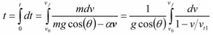
where v_t1 = mg cos(θ)/α is the terminal velocity. There is one other variable that describes the motion, and that is the characteristic time, τ₁ = m/α. The characteristic time is a measure of how quickly (or slowly) the object speeds up or slows down to the terminal velocity, and it shows up in the equations after we integrate. The formula for the quadratic drag model’s terminal velocity and characteristic time is different than the linear drag model’s characteristic time and terminal velocity. The linear drag models are labeled with subscript 1s. Another way to calculate the terminal velocity is to set the force equation to zero and solve for the velocity. This integral is evaluated with a change of variables x = 1 – v/v_t1, so that dx = – dv/v_t1.

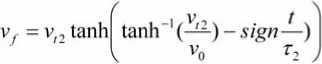
Lastly, we solve this somewhat intimidating equation for v_f, which turns out nicely as:

Equation 1. 

If you feel like practicing taking limits, see what happens when the air resistance coefficient goes to zero. The traditional v_f = v₀ + g cos(θ)t pops up. The first few terms in this expansion are useful if you want to approximate the exact solution in order to avoid the expensive exponential function calls.

For the quadratic case, we solve the equations in the same way. We start with the general equation:

From this equation we define the terminal velocity, , and the characteristic time is (not obvious from the equation) , which shows up after we integrate. Integrating this equation is straightforward. Although related, the plus version and the minus version are different integrals, and we need to evaluate both.

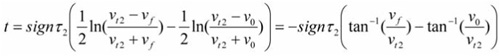
First, let us do the integral when the terminal velocity term (labeled with subscript 2s for the quadratic model) and the velocity square terms have the same sign. This is the case where the force of gravity and the fluid resistance are in the same direction, which happens when the particle is traveling up and both forces are pointing down.

To keep track of the overall sign relative to the velocity direction, we introduce the variable, sign, which is either 1 or –1, on the outside of the integral. This is important to get the correct overall sign compared to the direction of the velocity unit vector, . We continue to solve for the time as a function of initial and final velocity to obtain:

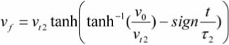
Now we solve this equation for the final velocity and obtain:

Equation 2. 

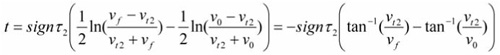
Secondly, we solve for the case where the terminal velocity and velocity squared terms have opposite signs:

There is a relevant connection between the inverse hyperbolic tangent and the natural log of the form:

The absolute value bars from the integral are important in order to get the equation to involve the inverse hyperbolic tangent correctly. We must answer whether the initial and final velocities are bigger than the terminal velocity. In addition, given that the initial velocity is less than the terminal velocity, is the final velocity necessarily less than the terminal velocity? It turns out that it is (see the solution below), and it is acceptable to convert both natural logarithms to inverse hyperbolic tangents. A similar question can be asked if the initial velocity is greater then the terminal velocity.

So there are four different cases with which we need to deal: V₀ <V_t2, V₀ > V_t2, V₀ = V_t2, and V_t2 = 0.

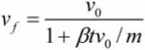
For the first case V₀ < V_t2:

and solving for the final velocity:

Equation 3a. 

For the second case V₀ > V_t2:

and solving for the final velocity:

Equation 3b. 

For the third case, v₀ = v_t2, where the object begins traveling at the terminal velocity in the same direction as the force of gravity, we get:

Equation 3c. 

There are several ways to arrive at this result. We can take a limit of both of the first two cases, Equations (3a) and (3b), or if we look at the force in the quadratic force equation, it is zero, hence the object must travel at a constant velocity.

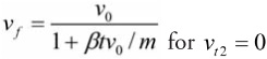
And lastly is the case when the terminal velocity is identically zero, V_t2 = 0. It is easiest to start from the original equation and solve like the previous cases.

As previously, we solve this for the final velocity:

Equation 3d. 

All right, this is all the information we need to solve for the linear and quadratic three-dimensional cases, and we now transition to solving the three-dimensional linear case.

We could solve the linear three-dimensional case in a similar manner as we solve the quadratic version. However, we choose to treat it as three separate one-dimensional problems because the results can be used by the AI in your game. The previous equations are modified to suit each of the Cartesian directions x, y, and z. Again, gravity is in the negative z direction. The solutions of the three different velocity equations are:

v_xf = v_x0 exp(–t/τ₁)

v_yf = v_y0 exp(–t/τ₁

and

v_zf = (v_z0 – v_tl)exp(– t/τ₁) + v_tl

with v_tl = –mg/α and τ₁ = m/α. The terminal velocities in the horizontal direction are zero.

If we integrate these equations with respect to time, then we get the position as a function of time.

x = v_x0 τ₁ (1 – exp(–t/τ₁) + x₀

y = v_y0 τ₁ (1 – exp(–t/τ₁)) + y₀

and

z = (v_z0 – v_tl)τ₁(1 – exp(–t/τ₁)) + v_tlt + z₀

The complete distance equations are useful for AI targeting, AI pathfinding, and calculating targeting info for players, without actually propagating the solutions forward in time step by step. In general, the distance equations are well approximated for most video games with x = x₀ + vt, since the time for most games is very small and is much faster than updating with the complete position equations.

The three-dimensional quadratic equations are , . It is impossible to solve these as three independent equations since they are all coupled by the quadratic term of the fluid resistance. One way to solve this is to break the motion into two directions, along the current velocity and perpendicular to the current velocity, and then update the velocity based on the force calculated.

Along the direction of motion, the force is F_parallel = –mgn_z – βv², where n_z is the z component of and is equal to negative of the cosine of the angle between the direction of motion and the gravity vector. Notice that the drag term is always negative since it is in the opposite direction as the current velocity.

Perpendicular to the direction of motion, the forces are . If the velocity is either straight up or straight down, n_z = ±1 and n_x = n_y, there is no component of force perpendicular to the current velocity. And if the velocity is completely horizontal, the perpendicular force is completely in the negative z direction. If you have a different coordinate system, this equation will look slightly different.

For the motion along the velocity normal, there are three different cases to consider: n_z> 0, n_z< 0, and n_z= 0. If n_z > 0, the object is moving upwards, the opposite direction from gravity, and the fluid resistance is in the same direction as gravity. If n_z< 0, then the object is moving in the same direction as gravity, and the fluid resistance force is in the opposite direction as gravity. Lastly, if n_z= 0, then the object is moving horizontally, and gravity has no effect on horizontal motion.

For n_z> 0, the relevant solution is Equation (2) with , , and sign = – 1 The velocity is:

For n_z < 0, the relevant solution is Equation (3a), (3b), (3c), or (3d) depending on the current velocity relevant to the current terminal velocity with , , and sign = – 1. The velocity update is:

or

Notice that the characteristic time for the last instance is undefined, but it is never used in the solution, so there should not be a problem.

For the force perpendicular to the initial velocity, the updated velocity is the same as Equation (3) with v₀= 0 and its own distinct terminal velocity, , and characteristic time, .

This leads to:

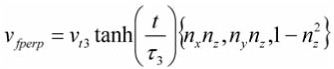
For most cases this can be approximated (since the characteristic time is usually large and the update time is usually small for games) as:

Equation 4. 

This last equation should look familiar. So usually there is no need to calculate the separate terminal velocity or the characteristic time for the perpendicular motion if the mentioned approximations are valid.

There is one issue that occurs when a slow-moving object changes from traveling upward to going downward, as shown in Figure 2.6.2. If this case is not handled, then the object appears to go back in the direction it came from, when in fact it would stop traveling in the horizontal direction and travel down along the direction of gravity.

Figure 2.6.2. A bad thing that can happen for slow-moving particles and/or large update times.

There are several ways to handle this. The most straightforward approach is to propagate the object for the time it takes to get to the top with Equation (2) and then for the rest of the time propagate with Equation (3a). From Equation (2), we can calculate the time it takes to stop moving in the positive velocity direction. The result is:

Equation 5. 

If the time to the top is less than the total time to propagate, then subtract the time to the top from the total time to propagate. Then use the downward velocity update for the time remaining and use zero as the initial velocity. There might be a slight discontinuity in the object’s smooth motion on the screen, but usually there is not. If there is too much, then update the position in a more rigorous manner.

The last thing to consider is how to update the position. All of these equations are integrable, which is more accurate, but they provide little extra accuracy noticeable in a gaming environment and are computationally expensive to evaluate. For most game purposes, it is accurate enough to use Euler integration to calculate the position X_f = X₀ + Vt, where the time, t, in the equation is the time since the last update and is not the global time. For the Golf Globe game on an iPod Touch, the game runs smoothly with no visible numerical issues at 60 frames per second by updating the position using Euler integration.

This is the pseudocode for a function that calculates the final velocity, velocityFinal, given the initial velocity, velocityInitial, of an object by the time, deltaTime. This does not update the position of the object, which should be updated separately but with the same deltaTime.

void updateVelocityWithFluidResistance(
      const float deltaTime,
      const ThreeVector& velocityInitial,
      ThreeVector& velocityFinal )
{
      Calculate Velocity Normal or zero it.
      Calculate terminal velocity and characteristic time along velocity
normal.

      For objects going up use Equation (2), but first check
to make sure the velocity does not reach the top
Equation (5).

      For objects going down use either Equation (3a), (3b),
(3c), or (3d) as is appropriate to the initial velocity at the
beginning of the frame.

      Update the velocity perpendicular to the initial velocity with
Equation (4).
}

There are benefits to using either the linear version or the quadratic version. The computational advantages lie with the linear solution. The quadratic computational cost is hardly prohibitive, especially if there are not too many objects updated with the quadratic model. And the quadratic model looks and feels much nicer, especially in a game where the user is getting feedback from movement due to handheld motion, such as from the iPod Touch or another handheld device.

There are several advantages to the linear solution: There are exact velocity and position equations for all time, which is useful for AI and targeting; it is faster computationally; and the exponent in the solution is easily expanded, making it only minutely more computationally intense than updates with gravity only.

One disadvantage to the linear solution is that it is not as realistic, especially when compared directly to the quadratic case.

There are some advantages to using the quadratic solution: It is more realistic and it is not hugely more computationally intense (as long as there are not too many objects). There are several disadvantages to the quadratic solution: It is computationally more intense, especially if there are many objects; there is no analytic solution for all time, thus it is not as easy to use for AI and player targeting; and its approximations are more difficult and are more numerically touchy to the input drag parameters.

There is a possible way to balance the two approaches if there are too many objects to update with the quadratic drag model. Use the linear model for the vast majority of these objects and then use the quadratic for the more important, or highly visible, objects.

For both the linear and the quadratic solutions, it is a good approximation to use Euler integration to update the object position. It will save big on computational cost if there are many objects, especially for the quadratic case.

The concept of drag is simple: Slow things down in the opposite direction they are moving. However, it is difficult to implement in a numerically accurate and stable manner. The simple and mathematically accurate linear drag model as presented here would be an improvement to many current games. The mathematically and physically accurate quadratic model is an additional improvement. There are many areas of simulation in games that would visibly benefit from using the mathematically and physically accurate quadratic drag model instead of the linear drag model: boats, sailboats (both with respect to the water and the wind in the sails), parachutes, car racing, snow-globe games, golf ball trajectories, craft flying through atmospheres, and artillery shells.

Along the lines of this gem, there are several areas that would be interesting to research further. Physically based drag coefficients depend on all sorts of factors, including temperature, density, type of fluid, and the shape of the object. For spacecraft entering an atmosphere, several of these things are relevant and can make for some interesting gameplay while flying into land or chasing AIs or other players in a multiplayer game.