
Introduction to Visual Basic for Applications
This entry is a brief introduction to Visual Basic for Applications (VBA), the programming language environment that allows Microsoft Excel users to automate tasks, create their own functions, perform complex calculations, and interact with spreadsheets. We focus on features of VBA useful for financial applications. For a comprehensive introduction to VBA, good references are Walkenbach (2004) and Roman (2002). The Excel VBA help is also useful as a quick reference. All Excel commands listed in this entry are based on Microsoft Office 2007.
A SIMPLE EXAMPLE OF A VBA PROGRAM
Before we review some important characteristics of the VBA language, let us create a simple example of a VBA program. Excel has a tool for recording tasks performed in a spreadsheet, which can then be replayed as a macro. Macros in Excel record a sequence of commands, so that you do not have to repeat the same set of instructions if you need to perform the task several times. Macros are in effect computer programs whose commands are hidden from the user, but can be seen if you open the VBA editor (VBE). You can access the VBE by using a shortcut, Alt-F11, in all versions of Excel. In Excel 2007, VBE can be accessed from the Developer tab. If the Developer tab is not visible, do the following to set it up: Click on the main MS Excel button ![]() , then Excel Options. Under the Popular Options tab, check Show Developer Tab in Ribbon. Once the Developer tab is available in Excel's top menu, you can click on the Visual Basic button in the ribbon associated with it to open the editor. (See Figure 1.)
, then Excel Options. Under the Popular Options tab, check Show Developer Tab in Ribbon. Once the Developer tab is available in Excel's top menu, you can click on the Visual Basic button in the ribbon associated with it to open the editor. (See Figure 1.)
Figure 1 Visual Basic Button in the Developer Ribbon in Excel 2007
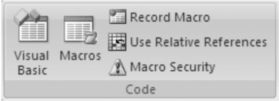
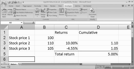
Figure 2 Macro Recording Example
Use the Macro Security button to enable macros. (It is always a good idea to return to the default—disabled macros—after you are finished working with macros.)
Open a new file and name it ReturnCalc.xlsm. (Excel 2007 will automatically make the file extension .xlsm if there are macros already in the file. Here, we do not have macros yet, so the default in Excel 2007 will be to save the file as .xlsx. To save the file with extension .xlsm, you need to select Excel Macro-Enabled Workbook from the drop-down menu next to Save as Type in the Save dialog box.)
We are trying to create the layout shown in Figure 2. First, enter the text in columns A and B; that is, enter stock prices for three points in time. Suppose we want to compute the realized cumulative return over the two time periods for any set of three stock prices in column B. We can do that by, for example, computing the realized returns over each of the two periods in column C, and then computing the cumulative return between times 1 and 3 in cell D5. Let us record the entries and the calculations as a macro. To record a macro, click on Record Macro in the Developer tab. Delete the default name Macro 1, and replace it with something more meaningful, for example, ReturnCalc. Click OK. Once the macro recorder is on, do the following:
Now let us see what the macro does. You can use the file you created. Delete all contents from the array C3:D5. Press Alt-F8 or, equivalently, click on the Macro button in the Developer tab. Select ReturnCalc, press OK. The spreadsheet
should fill up with the entries that you entered before. If you had changed the value of the stock price in any of the three cells in column B, the macro should calculate the correct corresponding value for total return in cell D5.
Behind the scenes, Excel recorded VBA code with instructions that tell Excel what functions to perform when you run the macro. You can see these instructions by opening the VBA editor and clicking on Modules | Module 1. The instructions look like this:
1 Sub ReturnCalc()
2 '
3 ' ReturnCalc Macro
4 ' Macro recorded month/day/year by you
5 '
6
7 '
8 Range("C3").Select
9 ActiveCell.FormulaR1C1 = "= (RC[-1]-R[-1]C[-1])/R[-1]C[-1]"
10 Range("C3").Select
11 Selection.Copy
12 Range("C4").Select
13 ActiveSheet.Paste
14 Range("C3:C4").Select
15 Selection.NumberFormat = "0.00%"
16 Range("D3").Select
17 ActiveCell.FormulaR1C1 = " = 1+RC[-1]"
18 Range("D3").Select
19 Selection.NumberFormat = "0.00"
20 Range("D4").Select
21 ActiveCell.FormulaR1C1 = " = R[-1]C*(1+RC[-1])"
22 Range("C5").Select
23 ActiveCell.FormulaR1C1 = "Total return"
24 Range("D5").Select
25 ActiveCell.FormulaR1C1 = " = R[-1]C-1"
26 Range("D5").Select
27 Selection.Style = "Percent"
28 Selection.NumberFormat = "0.00%"
29 Range("C5:D5").Select
30 Selection.Borders(xlDiagonalDown).LineStyle = xlNone
31 Selection.Borders(xlDiagonalUp).LineStyle = xlNone
32 Selection.Borders(xlEdgeLeft).LineStyle = xlNone
33 With Selection.Borders(xlEdgeTop)
34   .LineStyle = xlDouble
35   .Weight = xlThick
36   .ColorIndex = xlAutomatic
37 End With
38 Selection.Borders(xlEdgeBottom).LineStyle = xlNone
39 Selection.Borders(xlEdgeRight).LineStyle = xlNone
40 Selection.Borders(xlInsideVertical).LineStyle = xlNone
41 Range("D5").Select
42 End Sub
Knowing the actions we took to create the macro, it is relatively straightforward to trace what the program is doing at every step. To understand better how the macro works, however, and to know how to create such scripts without recording them in the spreadsheet, we need to understand some basic facts about VBA.
OBJECTS, PROPERTIES, AND METHODS
The most important fact about VBA is that it tries to act as an object-oriented language. (VBA does not quite qualify as an object-oriented language for technical reasons; however, for all practical purposes it is helpful to remember that VBA shares many of the same concepts as “real” object-oriented programming languages.) This means that it treats every component of Excel, such as a worksheet, a cell, a range of cells, and a chart, as an object. Objects are arranged in a hierarchy and have properties (attributes) that can be modified by entering the name of the object followed by dot and a specific command. In addition, objects are associated with actions (methods) that the objects can perform or have applied to them. You can view all objects by selecting View | Object Browser from the top menu in the VBE window. In Excel 2007, you can also view a detailed list of objects, their properties, and their methods by clicking on Help (pressing F1) and selecting Excel Object Model Reference.
The largest object, the object on top of the hierarchy, is Excel itself. It is the Application object. Worksheets, ranges, selections, charts, and so on are all objects that are lower in the hierarchy. Objects in the same class are organized in collections. For instance, the Workbooks collection contains all workbooks (Excel files) that are currently open. Similarly, the Worksheets collection contains all Excel spreadsheets in the files that are currently open, the Sheets collection contains all Excel spreadsheets and charts in the files that are currently open, and so on. Thus, for example, to reference cell C3 in Worksheet Return in file (Workbook) ReturnCalc.xlsm, you would type
Application.Workbooks("ReturnCalc
 .xlsm").Sheets("Return").Range("C3")
This reference is rather long and, as we can see from the actual VBA code, it is not necessary, as long as the macro is saved within the active Excel workbook and the identification of the cell range that is referenced is unique. In our example, Range("C3") is sufficient to reference cell C3, because the objects higher in the hierarchy, such as the name of the worksheet and the name of the file, are implied in the reference.
An example of an action (method) that can be performed on an object is the command Select. The Select method applies to several objects, including Worksheet, Chart, and Range. Notice that it was used often in the macro we created, because clicking on a cell or highlighting on an array performed the action. For example, in line 14 we selected the range C3:C4. Similarly, in line 10 we selected the cell C3 with the command
Range("C3").Select
Then, the Selection property of an object in the background (the Window object) was used to return a Range object (representing the selected range on the spreadsheet) on which we can apply other methods, such as Copy (line 11 of the code):
Selection.Copy
VBA usually suggests actions and properties that can be used with an object, so you can select from a list.
Another example of modifying the properties of the object is in lines 14–15 of the VBA code. They request that the format of the cell range C3:C4 be changed to percentage with two digits after the decimal point. Namely, we selected the range C3:C4, and the NumberFormat property of the Range object that was returned by the Selection property was set to percentage with two digits after the decimal point.
While the code we created by recording a macro is helpful in understanding the basics of the VBA language, it can be confusing because it is unnecessarily verbose. For example, the same result as lines 14–15,
Range("C3:C4").Select
Selection.NumberFormat = "0.00%"
can be achieved with the command
Range("C3:C4").NumberFormat =
 "0.00%"
which modifies directly the property NumberFormat of the object Range("C3:C4").
You can test that this is the case by deleting lines 14–15 in the VBA code in your file and replacing them with Range("C3:C4"). NumberFormat = "0.00%". Save the code by pressing Ctrl-S or selecting Save from the list under the main Excel button ![]() . Next, delete cells C3:D5 in the spreadsheet, and run the ReturnCalc macro again. The result and the formatting should be the same.
. Next, delete cells C3:D5 in the spreadsheet, and run the ReturnCalc macro again. The result and the formatting should be the same.
The effect of the With/End structure in lines 33–36 is another piece of code that can be replicated easily through other commands; the advantage of the structure is that it allows you to reduce the number of listed objects in the code, and that it makes the code more readable. A With/End statement requires the specification of an object. Inside the With/End statement, one can omit mentioning the object with every modification of a property or application of a method to the object. In this particular example, lines 33–36 could be replaced with
Range("C5:D5").Borders(xlEdgeTop)
 .LineStyle = xlDouble
Range("C5:D5").Borders(xlEdgeTop)
 .Weight = xlThick
Range("C5:D5").Borders(xlEdgeTop)
 .ColorIndex = xlAutomatic
with the same effect as the With/End statement that references Range("C5:D5"). Borders(xlEdgeTop). However, the With/ End statement is more concise.
In general, when writing VBA code you do not need to select cells explicitly in order to enter data into them. However, if you are new to VBA, it is helpful to record the macro first to see the code VBA suggests, and clean up afterward. In addition, it is a good idea to “comment out” the redundant statements at first, rather than deleting them. (Commenting out is done by entering an apostrophe (') at the front of the line of code that you wish VBA to ignore.) After commenting out overly verbose statements, save the macro by pressing Ctrl-S, make sure it still does what you would like it to do, and only then go back and delete the redundant statements.
A less verbose version of the VBA code is
Sub ReturnCalc()
'
' ReturnCalc Macro
' Less verbose
'
 Range("C3").Formula = "= (RC[-1]
 -R[-1]C[-1])/R[-1]C[-1]"
 Range("C3").Copy
 Range("C4").Select
 ActiveSheet.Paste
 Range("C3:C4").NumberFormat =
 "0.00%"
 Range("D3").Formula = "= 1+RC[-1]"
 Range("D3").NumberFormat = "0.00"
 Range("D4").Formula = "= R[-1]C*
 (1+RC[-1])"
 Range("C5").Formula = "Total
 return"
 Range("D5").FormulaR1C1 = "=
 R[-1]C-1"
 Range("D5").Style = "Percent"
 Range("D5").NumberFormat = "0.00%"
 With Range("C5:D5")
 .Borders(xlDiagonalDown)
 .LineStyle = xlNone
 .Borders(xlDiagonalUp)
 .LineStyle = xlNone
 .Borders(xlEdgeLeft).LineStyle
 = xlNone
  With .Borders(xlEdgeTop)
     .LineStyle = xlDouble
     .Weight = xlThick
     .ColorIndex = xlAutomatic
  End With
  .Borders(xlEdgeBottom).LineStyle
  = xlNone
  .Borders(xlEdgeRight).LineStyle
  = xlNone
  .Borders(xlInsideVertical)
  .LineStyle = xlNone
 End With
 Range("D5").Select
End Sub
Notice how the With/End structure was used to reduce the number of words we need to use, and how With/End structures can be nested inside one another. You can test that this code achieves the same effect by replacing the current code in the module in your file ReturnCalc.xlsm, saving the new code, and rerunning the macro ReturnCalc.
Before we end this section, we would like to mention a useful property of the Range object, Offset(v,h). It points to a cell that is v cells above or below (vertical direction) and h cells to the right or left (horizontal direction) from a specific cell. For example,
Range("C5").Select
ActiveCell.Offset(1,2) = 10
sets the value of the cell that is 1 cell down and 2 cells to the right from cell C5 (i.e., cell E6) to 10. Similarly,
Range("C5").Select
ActiveCell.Offset(-1,-2) = 20
sets the value of the cell that is 1 cell up and 2 cells to the left from cell C5 (i.e., cell A4) to 20.
We saw the idea of referencing cells above and below and to the left and right of the current cells in the example code at the beginning of this section. For example, the formula in line 9 of the original macro,
ActiveCell.FormulaR1C1 = "= (RC[-1]
 -R[-1]C[-1])/R[-1]C[-1]"
uses the cell in the same row and one column to the left (RC[-1]) and the cell one row up and one column to the left (R[-1]C[-1]) to compute the value in the active cell. These kinds of commands help when one prefers to create relative references—in other words, to perform tasks relative to a prespecified location in the spreadsheet without changing the code when the starting location is changed.
The default in VBA is to record macros in absolute reference mode. To change the mode to relative references, make sure that the relative references button in the Developer tab (![]() ) is “pressed in” before starting the macro recorder.
) is “pressed in” before starting the macro recorder.
PROGRAMMING TIPS
While some desired formatting of an Excel spreadsheet can be recorded with the macro recorder, knowing basic programming in VBA opens up a whole lot of additional functionality. For example, suppose that you have a set of data on stock returns over several months and, as often happens with real-world data, it is not recorded well—there are some duplicate rows. You could record a macro as you go through the spreadsheet and clean them by hand, but next time you have a set of data, duplicate entries will not be exactly in the same rows as the first set of data. How can you tell Excel to sort through the data and remove duplicate rows in any set of data? You need to construct a program from scratch and make the code general enough to enable the script to be transferable.
In the remainder of this section, we cover some basic VBA programming concepts. We discuss the difference between subroutines and user-defined functions, explain variable declaration in VBA, and introduce some important control flow statements. These concepts are not unique to VBA—versions of them exist in most programming languages.
Subroutines versus User-Defined Functions
Subroutines and user-defined functions in VBA are both blocks of code saved in modules. (If you do not see a module when you open VBE, select Insert | Module from the top menu in VBE to create one.) The difference is that subroutines are general scripts; that is, lists of instructions, whereas functions complete a list of instructions and return a value to the user. Subroutines have the general form
Sub ()
[commands]
End Sub
whereas functions have the form
Function FunctionName(list of inputs)
 As type [commands]
FunctionName = Return value
 'Computed from [commands]
End Function
The macro recorded at the beginning of this entry was an example of subroutine code. Next, we provide another small example in order to illustrate the difference between a subroutine and a function. Do not worry about the details of the commands right now; we will explain each part of the code in subsequent sections.
Suppose we would like to calculate n! (pronounced “n factorial”), where n is an integer number the user provides as input. n! is the product of all integer numbers less than or equal to n; that is, n! = 1·2·…·n. Next, we provide several examples of subroutines and user-defined functions that accomplish this goal. The subroutine
Sub FactorialSub1()
'Compute factorial using control flow
 statements
 'Declare the variable that will
 'store the value for factorial
 Dim Factorial As Integer
 'Declare the variable that will
 'store the number n
 Dim inNumber As Integer
 'Declare the variable that will be
 'used as counter in the loop
 Dim i As Integer

'Read in the number from cell B1,
'store it in inNumber
 inNumber = Range("B1").Value

 'Calculate factorial
 Factorial = 1
For i = 1 To inNumber
 Factorial = i * Factorial
Next i

  Range("B2").Value = Factorial
End Sub
takes the number specified in cell B1, computes the factorial of that number, and sets the value of the cell B2 to the value of that factorial. To see how this subroutine works, copy the code in a new module in the VBE window of a new Excel file. Enter the number 5 in cell B1. Press Alt-F8, and select FactorialSub1. The subroutine fills cell B2 with 120 (5! = 1·2·3·4·5 = 120).
The function FactorialFun1 whose code is provided next computes the same result, but works in a different way. It takes a number as an input (inNumber), and returns a number as an output (FactorialFun1). The output to be returned should have the same name as the function.
Function FactorialFun1(inNumber)
 As Integer
 Dim i As Integer
 'Calculate factorial
 FactorialFun1 = 1
 For i = 1 To inNumber
 FactorialFun1 = i * FactorialFun1
 Next i
End Function
Add this function to the module in the VBE in your file. To call this function, type in a cell in your spreadsheet (say, cell B3) = FactorialFun1(B1). If the value in cell B1 was still 5 (the value you entered in the previous example), then the value of cell B3 will be 120. Notice that the syntax for calling your (user-defined) function is not different from the syntax for calling built-in Excel functions. In fact, Excel has a function for computing a factorial, = Fact(number), and if you entered the expression = Fact(B1) in, say, cell B4 of your spreadsheet, you would get the same result (120).
Excel built-in functions can be used also inside VBA code with the prefix Application. It is worthwhile to note, though, that VBA itself has some built-in numeric functions. In particular, functions such as Abs (absolute value), Exp (exponential), Int (integer part), Cos (cosine), Sin (sine), Log (natural log), Rnd (random number generator), Sign (sign function), Tan (tangent), and Sqr (square root) can be used directly within VBA code without the prefix Application. Although it seems that this should make things easier, it may also be a source of confusion. Notice that Excel has equivalent numerical functions for formulas that are entered into cells in spreadsheets, but the syntax for some of the functions is different. For example, the natural logarithm function in Excel is Ln, and the square root function is Sqrt. So, typing Sqr in your program in VBA is equivalent to typing Application.Sqrt. In practice, you would want to use the shorter syntax Sqr. It is important to be aware of inconsistencies between names of equivalent functions in Excel and VBA.
The subroutine FactorialSub1() and the function FactorialFun2() whose code is provided below illustrate how the factorial can be computed by calling the built-in Excel function Fact.
Sub FactorialSub2()
'Compute factorial using Excel's FACT
'function within a subroutine
 Range("B5") = Application.Fact_
 (Range("B1"))
End Sub

Function FactorialFun2(inNumber) As
Integer
 'Calculate factorial
 FactorialFun2 = Application_
 .Fact(inNumber)
End Function
Copy the code above in the module in your file. The subroutine FactorialSub2() uses the number entered in cell B1 in the spreadsheet as an input and calls the Excel function Fact() to compute the factorial of the value in cell B1. The function FactorialFun2() is called with an input argument that is a number and returns the factorial of that number. If you type = FactorialFun2(B1) in cell B6 and the value in cell B1 is still 5, you should obtain 120 in cell B6.
What is the advantage of using user-defined functions rather than subroutines? In some cases, you can only use one or the other. However, in cases in which both are possible, it may be preferable to structure the script as a function as opposed to a subroutine. User-defined functions are more “transferable”—in other words, it is easier to use them in different places in the spreadsheet. There are some other conveniences—for example, check what happens when the number for n in cell B1 is changed from 5 to 6. Cell B3 (which contains the call to the function FactorialFun1) immediately updates to 720, which is the correct result. However, cells B2 and B5—those that are output ranges for the subroutines FactorialSub1 and FactorialSub2—do not update until you rerun the macros associated with them.
Variable Declaration
Variables are a basic common concept in computer languages. They are used to store numerical and text data and handle intermediate output in subroutines and functions. For example, inNumber in the code for FactorialSub1 was a variable that stored the value of n for which the factorial should be computed. There is no convention for naming variables, but a good practice is to give them meaningful names (rather than x, y, and z), so that your code is easier to follow. We prefer to start names of variables with small letters. If there is a second word in the name, that word starts with a capital letter. We also like to differentiate variables that store inputs (such as inNumber) and variables that record output (e.g., outFactorialValue).
Depending on their type, variables are handled differently and are allocated a different amount of memory. For example, we specified that inNumber should be an integer number by declaring it with the syntax Dim variableName As variableType:
Dim inNumber As Integer
Other types of variables include String, Single, Double, Long, Boolean, Date, Object, Variant, and so on. For example, when you need a variable that will hold a fractional (also called “floating point”) value, then you should use the Single or Double data type. When you need a variable to store text data, use the String type. The Variant type can be used to replace any type; however, it also uses up the largest amount of space, so it is better to specify a particular type for a variable if you know it.
When specifying a variable type, make sure that you have enough space for the data you are planning to store in that variable. If the value gets too large for the variable type, your program may crash. For example, the Integer type can store values between –32,768 and 32,767. If you need to store an integer number outside this range, use the Long variable type. Similarly, the Single (floating point) type can store numbers between –3.402823E38 and –1.401298E-45 for negative values, and numbers between 1.401298E-45 and 3.402823E38 for positive values.1 If you need to work with fractional numbers outside this range, use the Double (floating point) variable type.
Variables can be grouped into arrays. For example,
Dim myArray(5) As Integer
declares an array of integers of size 6.
One of the most confusing things about VBA is the way it handles arrays. The default is to index the first element in arrays as 0, which is the convention in most programming languages, which is why the total number of elements in myArray is 6. However, in some special circumstances arrays are treated as starting with the index 1. To ensure consistency and minimize confusion, it is helpful to use the command
Option Base 1
at the beginning of the module, which makes sure that the indexing of arrays always starts at 1. If this option is stated, then declaring
Dim myArray(5) As Integer
will result in an array of 5 elements. Those elements can be referenced as myArray(1),…, myArray(5) later in the program.
You can specify arrays of multiple dimensions as well, for example,
Dim myMultiArray(5,2) As Integer
will result in an array of 5 rows and 2 columns.
You can also declare dynamic arrays, that is, arrays that do not have specific dimensions from the beginning. This may happen if, for example, you have a set of data and you need to read it in before you know how many elements it has. In that case, you would declare an array
Dim myDynamicArray() As Integer
which will be filled as necessary. Once the number of elements is counted, the array can be resized by using the command ReDim, for example,
ReDim myDynamicArray(10)
ReDim reinitializes (sets to empty) all values within an array. If you want to preserve the values that are already there, use ReDim Preserve, which preserves as many elements as can fit in the new array dimensions.
Working with arrays within VBA is cumbersome and prone to errors. Often, one needs to resort to loops (see the introduction to loops in the next section) to handle array operations. In many cases, it may be preferable to use built-in Excel array manipulation functions, such as SUMPRODUCT, which performs vector multiplication. As we mentioned earlier, such built-in Excel functions can be called with Application.FunctionName. For example, Array3 = Application.SUMPRODUCT(Array1, Array2) will fill a variable array Array3 with the result of the elementwise multiplication and summation of the matrix arrays Array1 and Array2.
VBA will assume that you are creating a new variable whenever you use an expression that is not one of the standard commands. Stating the type of variables you use in the program can save you a lot of headache. (Typically, variable declaration is done at the beginning of the program.)
We also strongly recommend that you write the statement Option Explicit in the first line of your modules. This statement makes sure that Excel will report an error if it encounters an undeclared variable in your code. (This also can be accomplished by checking Require Variable Declaration under Tools | Options in the top VBE menu.) While this may seem like an inconvenience, think about a situation in which you mistype the name of a variable somewhere in your program. If Excel is not in the Option Explicit mode, it will treat the mistyped name as a new variable, ignoring any value that your variable may have had at that point in the program, and you will get nonsensical output. If Excel reports an error instead, you will know to fix the typo.
Control Flow Statements: For and If
Control flow statements in VBA allow for building more sophisticated programs than simple input and output of data to Excel. We briefly review a couple of important control statements that are used in VBA code: an example of an iterative statement (the For loop) and an example of checking a condition (the If statement).
The general syntax of a For loop in VBA is as follows:
For i = 1 to n
commands
Next i
The commands inside the For loop are executed once for every value of n. (One can also specify a step by writing For i = 1 to n Step k. For example, if n = 10 and step k = 2, then the commands in the loop will be executed for n = 1, 3, 5, 7, 9.)
We saw an example of a For loop in the code for calculating the factorial of a number n. Let us walk through the For loop code inside FactorialSub1.
 'Calculate factorial
   Factorial = 1
 For i = 1 To inNumber
  Factorial = i * Factorial
Next i
The initial value of Factorial is set to 1. Suppose the value for inNumber is 5. The loop starts at i = 1. During the first iteration, the new value of Factorial equals the current value of i (which is 1) times the current value of Factorial (which is 1 as well). At the end of the first run through the loop, the value of Factorial is 1. Next, the value of i is set to 2. The new value of Factorial equals the current value of i (which is 2) times the current value of Factorial (which is 1); that is, it equals 2. At the third iteration, the value of i is 3 and the current value of Factorial is 2; that is, the new value of Factorial is 3·2 = 6. And so on and so forth for the next values of i, which are 4 and 5. The value of Factorial keeps getting updated until it reaches 720 ( = 5!) in the last iteration of the loop.
There are other commands that enable iterating through commands multiple times, such as the Do While and Do Until. See VBE's Help for description of the syntax and use of these alternatives.
The general form of the If statement is
If condition Then
 commands
End If
When the condition is true, the block of commands executes. More generally, you can use a statement of the kind
If condition1 Then
   commands1
ElseIf condition2 Then
   commands2
Else
   commands3
End If
Commands1 will be executed if condition1 is true. If condition1 is not true, then (and only then) condition2 will be checked. If condition2 is true, then commands2 will be executed. If condition2 is not true, then commands2 will be executed.
When using If statements, one typically needs to compare values of variables and check whether conditions are true. Therefore, it is useful to know about the logical operators that allow for such comparisons and checks. The comparison operators are the following:
| = | tests for equality |
| <> | tests for inequality |
| < | tests whether the variable to the left of it is less than the variable on the right |
| > | tests whether the variable to the right of it is less than the variable on the left |
| < = and > = | test for less than or equal to/greater than or equal to |
Additional useful operators are AND, OR, and NOT. AND allows checking whether more than one statement is true at the same time. OR returns a True result if at least one of the statements is true. NOT returns a True result if the statement is false.
To illustrate how we can use these operators, consider a couple of simple examples that involve three numerical variables, var1, var2, and var3. Let var1 = 5, var2 = 10.
The code
If (var1 <> var2) Then
   var3 = 100
Else
   var3 = -100
End If
checks whether the value for var1 is different from the value of var2. If it is (i.e., the value of the logical statement (var1 <> var2) is True), then the value of var3 is set to –100; otherwise the value of var3 is set to 100. In this example, the value of var3 at the end of the loop is 100, since the value for var1 (5) is indeed different from the value of var2 (10).
Consider also the example
If (var1 < 5) Or (var2 > = 7) Then
  var3 = 100
Else
  var3 = -100
End If
The code checks if at least one of the statements (var1 < 5) and (var2 > = 7) is true. If at least one of them is true, then the value of var3 is set to 100; otherwise the value of var3 is set to –100. In our case, the first statement is false, because the value of var1 is not less than 5 (it is equal to 5). However, the second statement is true: The value of var2 (10) is indeed greater than or equal to 7. Therefore, the combined statement (var1 < 5) Or (var2 > = 7) is true, and the value of var3 will be set to 100.
User Interaction in VBA
While we covered the most fundamental concepts about the VBA language, it is fun to learn about some additional capabilities that enable your programs to interact better with their users. For example, once you have created a macro, you can associate it with a button that the user can press every time he or she wants the macro to run. To do that, go to the Developer tab, select Insert | Form Controls, and click on the button. When Excel pops up in the Macro dialog box, click on the macro you would like to have associated with this button.
Sometimes, it is convenient to ask the user to input information through an input dialog box. This can be done with the command InputBox("question for user", "title of the input box"). For example,
inNumber = InputBox("Enter an
integer", "Factorial Calculation")
will prompt the user to enter an integer number and will save that number into the variable inNumber. The title of the input box will be Factorial Calculation.
Other useful user interaction tools include Message Box ( MsgBox), which allows you to report output not in a cell on the spreadsheet, but in a message box. To test how it works, let us go through the following modification of the factorial calculation program (save it in your file as subroutine FactorialSubMsgBox()):
1 Sub FactorialSubMsgBox()
2 Dim inNumber As Variant
3 Dim numberType As Boolean
4 Dim outFactorial As Integer
5
6 inNumber = InputBox("Enter an integer number", "Factorial Calculation")
7
8 numberType = IsNumeric(inNumber)
9
10 If numberType = True Then
11   outFactorial = Application.Fact(inNumber)
12   MsgBox ("The factorial of " & inNumber & " equals " & outFactorial)
13 ElseIf numberType = False Then
14  MsgBox ("Not a number. Please enter an integer number.")
15 End If
16 End Sub
On line 6, we ask the user to specify the number for which we want to compute the factorial. On line 8, we check whether this is indeed a number. Note that the variable numberType is specified as Boolean, which means that it can only take True or False values. If it is true, that is, if inNumber is indeed a number, then we call the Excel built-in function Fact to calculate the factorial of this number, and print the statement “The factorial of the number the user entered is the result obtained” in a message box on the screen. If it is not true, then we prompt the user to enter a number.
Note that in line 2, we specified the type of variable for inNumber as Variant, which allows it to be anything. If we had declared inNumber As Integer and had entered a letter instead of a number, Excel itself would have returned an error, complaining that there is a variable type mismatch between what was declared and what the actual value of the variable is. Thus, declaring the exact type of variable whenever we know the type is very is important for minimizing errors in output.
DEBUGGING
VBA has useful debugging tools that allow you to look at the code in more detail if your programs do not work as expected. These tools can be accessed through commands under the Debug item in the top menu of the VBE.
The “Step Into” button ![]() (shortcut F8) lets you execute your program step by step. When you are executing a program step-by-step, your program is in “break mode.” Every time you press F8, the “break” is moved to the next command. While the break is set on a particular command, placing the cursor over any variable above the break point will give you an updated stored value for that variable. This makes it easy to catch calculation errors and inconsistencies. You can “step over” (i.e., skip) some subroutines that you are not interested in double-checking (use the button
(shortcut F8) lets you execute your program step by step. When you are executing a program step-by-step, your program is in “break mode.” Every time you press F8, the “break” is moved to the next command. While the break is set on a particular command, placing the cursor over any variable above the break point will give you an updated stored value for that variable. This makes it easy to catch calculation errors and inconsistencies. You can “step over” (i.e., skip) some subroutines that you are not interested in double-checking (use the button ![]() or the shortcut Shift-F8) and “step out” of the break mode (use the button
or the shortcut Shift-F8) and “step out” of the break mode (use the button ![]() or the shortcut Ctrl-Shift-F8). Equivalently, you can click on the Reset button in the top VBE menu (
or the shortcut Ctrl-Shift-F8). Equivalently, you can click on the Reset button in the top VBE menu (![]() ) to get out of debug mode.
) to get out of debug mode.
Rather than going through the program step-by-step, it is sometimes helpful in long programs to set breakpoints in advance, so that the program runs until it gets to a particular breakpoint. A breakpoint can be specified by placing the cursor at the place where it should be inserted, and clicking on the button ![]() in the Debug menu (or using the shortcut F9). When the program gets to the breaking point, it automatically goes into break mode and allows you to follow the subsequent commands step-by-step and check the values of the variables at that point in the program. To remove a breakpoint, simply place the cursor in the corresponding line, and click on the breakpoint button again.
in the Debug menu (or using the shortcut F9). When the program gets to the breaking point, it automatically goes into break mode and allows you to follow the subsequent commands step-by-step and check the values of the variables at that point in the program. To remove a breakpoint, simply place the cursor in the corresponding line, and click on the breakpoint button again.
EXAMPLES
The best way to learn to program in VBA is to see and implement many examples. Let us discuss three examples of using VBA in financial applications. The first example is a function that computes the Black-Scholes price of a European call option. It shows how a function is created, how variables are declared, and how Excel functions are accessed from within VBA. The second example is a function that generates possible paths for an asset price assumed to follow geometric Brownian motion. It involves using the random number generator in VBA, manipulating arrays, and iterating with loops. The third example is a function that computes the price of a European call option by simulation. It illustrates how user-defined and Excel functions can be called from within VBA functions, and provides another example of array manipulation and loops in VBA. Further examples of VBA scripts for financial applications, such as calculating the price of an Asian option, or computing and graphing the mean-variance efficient portfolio frontier (see Markowitz, 1952), can be found in Pachamanova and Fabozzi (2010). See also Jackson and Staunton (2001).
Pricing a European Call Option with the Black-Scholes formula
The Black-Scholes formula for a European call option (C) is as follows (Black and Scholes, 1973):
![]()
where
K
is the strike price
T
is the time to maturity
q
is the percentage of stock value paid annually in dividends
Φ
denotes the cumulative probability density function for the normal distribution
The value for Φ(d) can be found in Excel by using the built-in formula =NORMDIST(d,0,1,1) or, equivalently, the formula =NORMSDIST(d).
To illustrate the Black-Scholes option pricing formula, assume the following values:
Figure 3 Example of Using the User-Defined Function BSCallPrice in a Spreadsheet

Plugging into the formula, we obtain

Next, we provide the code of a VBA function that computes the price of a European call option with the Black-Scholes formula.
Function BSCallPrice(initPrice As_
 Double, _
	 	 K As Double, _
	 	 T As Double, _
	 	 r As Double, _
	 	 sigma As Double, _
	 	 q As Double)
'Computes the Black-Scholes price of a 'European call option
'initPrice is the initial price of the 'stock
'r is the interest rate
'T is the time to maturity of the 'option
'sigma is the volatility of the stock
'q is the continuous dividend yield

Dim dOne As Double

dOne = (Log(initPrice / K) + (r - q _ + 0.5 * sigma ^ 2) * T) / _
(sigma * Sqr(T))

BSCallPrice = initPrice * Exp(-q * T)_
 * Application.NormSDist(dOne) - _
K * Exp(-r * T) * Application. _
NormSDist(dOne - sigma * Sqr(T))


End Function
In the code above, all input variables (initPrice, r, T, sigma and q) are specified to be of type Double. A variable dOne is declared as type Double within the function. dOne stands for d1 in the definition of the Black-Scholes formula above. It takes the value of the expression (Log(initPrice / K) + (r - q + 0.5 * sigma ^ 2) * T) / (sigma * Sqr(T)). (Note that this expression contained an underscore (“_”) in the code above. The underscore is used when transferring a part of an expression to a new line.) The price of the option is stored in BSCallPrice. The functions Log and Exp used in the calculation are VBA functions. We also call the Excel function NormSDist with the expression Application.NormSDist.
The function BSCallPrice can then be used in a spreadsheet. An example is given in Figure 3. The inputs are stored in cells B3:B8, and the function is called with arguments that are cell references to cells where the information is stored.
VBA is forgiving if you are sloppy in writing the function. For example, the code below (without any variable declarations) would have worked as well.
Function BSCallPrice(initPrice,K,T,r,
sigma,q)

dOne = (Log(initPrice / K) + (r - q
+ 0.5 * sigma ^ 2) * T) / _ (sigma
* Sqr(T))

BSCallPrice = initPrice * Exp(-q * T)
 * Application.NormSDist(dOne) - _
K * Exp(-r * T) * Application.
NormSDist(dOne - sigma * Sqr(T))

End Function
However, as we mentioned earlier, it is a good practice to keep your code well organized. It helps minimize errors and saves you time in the long run.
Generating Paths for the Price of an Asset That Follows Geometric Brownian Motion
In finance, the dynamics of asset price processes in discrete time increments are typically described by two kinds of models: trees (such as binomial trees) and random walks. When the time increment used to model the asset price dynamics becomes infinitely small, such processes are referred to as stochastic processes in continuous time. The ability to generate paths for asset prices following these processes is important for computing prices of securities that depend on the asset price under consideration, as well as for calculating various risk measures associated with holding the asset in a portfolio.
The most widely used stochastic process in finance is geometric Brownian motion. The evolution of the underlying asset price is described by the equation
![]()
where Wt is standard Brownian motion, and μ and σ are the drift and the volatility of the process, respectively. (See a more detailed introduction in Hull [2008] or Pachamanova and Fabozzi [2010].) It turns out that the value of the asset price ST at time T given the asset price St at time t can be computed as
![]()
where ![]() is a standard normal random variable. If the stock pays a continuously compounded dividend yield of q, then we use (μ – q – 0.5·σ2) instead of (μ – 0.5·σ2) in the above formula.
is a standard normal random variable. If the stock pays a continuously compounded dividend yield of q, then we use (μ – q – 0.5·σ2) instead of (μ – 0.5·σ2) in the above formula.
Let us create a function, GBMPaths, that generates a prespecified number of paths (numPaths) for the asset. Each path consists
of a prespecified number of steps (numSteps). The value of the asset at each step is computed according to the formula for ST above. In the formula, we replace time t with time 0 (i.e., the present), and time T with the time corresponding to the step.
The code of the function is
Function GBMPaths(initPrice As Double, _
         mu As Double, _
         sigma As Double, _
         T As Double, _
         q As Double, _
         numSteps As Integer, _
         numPaths As Integer)
 Randomize
 Dim iPath, iStep As Integer
 Dim paths() As Variant
 ReDim paths(1 To numSteps + 1, 1 To numPaths)
  For iPath = 1 To numPaths
    paths(1, iPath) = initPrice
    For iStep = 2 To numSteps + 1
      paths(iStep, iPath) = paths(iStep - 1, iPath) * _
         Exp((mu - q - 0.5 * sigma ^ 2) * (T / numSteps) + _
         sigma * (T / numSteps) ^ (1 / 2) * _
         (Application.NormSInv(Rnd)))
 Next
 Next
 GBMPaths = paths
End Function
Let us now see what this function does. First, we use the command Randomize to make sure that VBA creates a different sequence each time we generate normal random variables to compute the paths for the asset. (If you do not type Randomize before you use the VBA random generator function Rnd, Rnd will always return the same sequence of numbers.)
Next, we declare variables we will use in the function. The variables iPath and iStep will be counters for the number of paths and the number of steps we have generated so far. They are, of course, integers. The two-dimensional array paths will store the values of the asset
along each path and for each step. We use ReDim to specify the dimensions of the array.
We next use a for loop to populate the array paths. In fact, we have two nested for loops—one that iterates through the number for paths, and one that iterates through the points in each path. For each point iStep on each path iPath, we calculate the price of the asset and store it in paths(iStep,iPath). The formula that computes the price of the asset contains the expression Application.NormSInv(Rnd), which generates a value for the normal random variable ![]() in the formula for ST earlier in this section. Rnd is the VBA random number generator—it returns a random number between 0 and 1. The reason we used the command Randomize at the beginning of the function is so that we could force Rnd to generate different sequences of random numbers every time you call the function GBMPaths. NormSInv is an Excel function that finds the number on the horizontal axis of the normal distribution that corresponds to the value for cumulative probability generated by Rnd. (See, for example, Chapter 4 in Pachamanova and Fabozzi [2010] for an explanation of how random numbers from different probability distributions are generated.) As in the previous example, in order to indicate to VBA that NormSInv is an Excel function, we use Application. in front of NormSInv.
in the formula for ST earlier in this section. Rnd is the VBA random number generator—it returns a random number between 0 and 1. The reason we used the command Randomize at the beginning of the function is so that we could force Rnd to generate different sequences of random numbers every time you call the function GBMPaths. NormSInv is an Excel function that finds the number on the horizontal axis of the normal distribution that corresponds to the value for cumulative probability generated by Rnd. (See, for example, Chapter 4 in Pachamanova and Fabozzi [2010] for an explanation of how random numbers from different probability distributions are generated.) As in the previous example, in order to indicate to VBA that NormSInv is an Excel function, we use Application. in front of NormSInv.
The function returns a two-dimensional array, GBMPaths (which is equal to paths, as set in the second-to-last line of the function). Every column of the array contains a randomly generated path for the asset price; that is, it has numSteps values that represent the values of the asset price along that path.
Pricing a European Call Option by Simulation
Let us now use the function we created in the previous section to write a function that prices a European call option by simulation. While this is not the most efficient way to price a European call option by simulation, it will illustrate how user-defined functions are called within other functions, and how arrays are handled as outputs of a function.
As in the previous section, we will make the assumption that the asset price follows geometric Brownian motion, which means that the value of the asset price ST at time T given the asset price St at time t can be computed as
![]()
where ![]() is a standard normal random variable. (When we generate asset price paths for the purpose of valuing an option, we use r (the risk-free rate) in place of the drift term μ. This is done for technical reasons (absence of arbitrage).) As in the previous section, if the stock pays a continuously compounded dividend yield of q, then we use (r – q – 0.5·σ2) instead of (r – 0.5·σ2) in the formula above.
is a standard normal random variable. (When we generate asset price paths for the purpose of valuing an option, we use r (the risk-free rate) in place of the drift term μ. This is done for technical reasons (absence of arbitrage).) As in the previous section, if the stock pays a continuously compounded dividend yield of q, then we use (r – q – 0.5·σ2) instead of (r – 0.5·σ2) in the formula above.
The price of the option can be approximated by creating scenarios for the stock price ST at time to maturity T, computing the discounted payoffs of the option, and finding the expected payoff of the option. (Option pricing by simulation was first suggested by Boyle, 1977. See also Boyle et al., 1997; Pachamanova and Fabozzi, 2010; Glasserman, 2004; or McLeish, 2005.)
Suppose we generate N scenarios for ![]() at time T:
at time T: ![]() (1),…,
(1),…, ![]() (N). Then, the price of a European call option with strike price K will be
(N). Then, the price of a European call option with strike price K will be
The expression above is the expected value of the option payoffs, that is, the weighted average of the option payoffs.
The VBA code of the function is given below.
Function EuropeanCall(initPrice As Double, _
           K As Double, _
           r As Double, _
           T As Double, _
           sigma As Double, _
           q As Double, _
           numSteps As Integer, _
           numPaths As Integer)
    Dim iPath As Integer
    Dim payoffs() As Variant
    ReDim payoffs(1 To numPaths)
    Dim paths() As Variant
    ReDim paths(1 To numSteps + 1, 1 To numPaths)

    paths = GBMPaths(initPrice, r - q, sigma, T, q, numSteps, numPaths)
    For iPath = 1 To numPaths

      payoffs(iPath) = Exp(-r * T) * _
      Application.Max(paths(numSteps + 1, iPath) - K, 0)
   Next

   EuropeanCall = Application. Average(payoffs)
End Function
The variable declarations are similar to the declarations in the previous sections; however, now we have an additional array, payoffs, that will store the payoff of the option at the end of each generated path (that is, for each generated scenario). The dimension of the array is therefore 1× numPaths.
After declaring the variables in the function, we call the function we created in the previous section, GBMPaths, and store the output in the array paths. This is achieved with the command
paths = GBMPaths(initPrice, r - q,
 sigma, T, q, numSteps, numPaths)
The arguments of the function GBMPaths were initPrice, mu, sigma, T, q, numSteps and numPaths. Note that when we call the function GBMPaths from within the function EuropeanCall, we input r - q in place of the argument mu.
After generating numPaths paths for the price of the underlying asset, we compute the payoffs of the option. We only need the payoffs at the time of maturity of the option, time T, so we only use paths(numSteps + 1, iPath) in the calculation.
The payoff along path iPath is calculated as the maximum of zero and the difference between the strike price K and the value of the underlying at the end of path iPath at time T.
We use the Excel function Max to compute the maximum and call it as Application.Max. Each payoff is discounted, and is added to the array payoffs.
After the array payoffs is filled, we compute the average of the payoffs to get the price of the option. We use the Excel function Average, which we call with the command Application.Average.
KEY POINTS
- Macros contain prerecorded tasks that can be performed in a spreadsheet. Macros are in effect computer programs whose commands are hidden from the user, but they can be seen if the VBA editor is open.
- The most important fact about VBA is that it tries to act as an object-oriented language. This means that it treats every component of Excel, such as a worksheet, a cell, a range of cells, and a chart, as an object.
- Objects are arranged in a hierarchy and have properties (attributes) that can be modified by entering the name of the object followed by a dot and a specific command. In addition, objects are associated with actions (methods) that the objects can perform or have applied to them.
- Subroutines and user-defined functions in VBA are both blocks of code saved in modules. The difference is that subroutines are general scripts; that is, lists of instructions, whereas functions complete a list of instructions and return a value to the user.
- Variable types in VBA include Integer, String, Single, Double, Long, Boolean, Date, Object, and Variant. A different amount of memory is allocated to storing values of variables of different types.
- The default in VBA is to index the first element in arrays as 0, which is the convention in most programming languages. The command Option Base 1 at the beginning of a module makes sure that the indexing of arrays starts at 1.
- Control flow statements such as For and If allow for building more sophisticated programs than simple input and output of data to Excel.
- Excel functions can be accessed from VBA by prefixing them with Application.
- VBA has some built-in numeric functions, but it is important to know that their syntax is not always the same as the syntax of the same function in Excel. For example, the function Sqrt (square root) in Excel is Sqr in VBA.
- Useful tools in Excel and VBA that allow for interaction with users include buttons, input dialog boxes, and message boxes.
- VBA has debugging tools that allow you to look at the code in more detail if your programs do not work as expected. These tools can be accessed through commands under the Debug item in the top menu of the VBE.
NOTE
1The notation E in Excel denotes multiplication by 10 to a specific power. For example, 5E40 means 5·1040, and 5E-45 means 5·10−45.
REFERENCES
Black, F., and Scholes, M. (1973). The pricing of options and corporate liabilities. Journal of Political Economy 81, 3: 637–654.
Boyle, P. (1977). Options: A Monte Carlo approach. Journal of Financial Economics 4, 3: 323–338.
Boyle, P., Broadie, M., and Glasserman, P. (1997). Monte Carlo methods for security pricing. Journal of Economic Dynamics & Control 21: 1267–1321.
Glasserman, P. (2004). Monte Carlo Methods in Financial Engineering. New York: Springer-Verlag.
Hull, J. (2008). Options, Futures and Other Derivatives, 7th ed. Upper Saddle River, NJ: Prentice Hall.
Jackson, M., and Staunton, M. (2001). Advanced Modelling in Finance Using Excel and VBA. Hoboken, NJ: John Wiley & Sons.
Markowitz, H. (1952). Portfolio selection. Journal of Finance 7: 77–91.
McLeish, D. (2005). Monte Carlo Simulation and Finance. Hoboken, NJ: John Wiley & Sons.
Pachamanova, D. A., and Fabozzi, F. J. (2010). Simulation and Optimization in Finance: Modeling with MATLAB, @RISK, and VBA. Hoboken, NJ: John Wiley & Sons.
Roman, S. (2002). Writing Excel Macros with VBA, 2nd ed. Sebastopol, CA: O’Reilly Media.
Walkenbach, J. (2004). Excel 2003 Power Programming with VBA. Hoboken, NJ: John Wiley & Sons.