Introduction to Financial Model Building with MATLAB

DESSISLAVA A. PACHAMANOVA, PhD

Associate Professor of Operations Research, Babson College

MATLAB is an interactive computing environment for model development that also enables data visualization, data analysis, and numerical simulation. The core of the MATLAB environment was created as a number-array-oriented programming language; that is, as a programming language in which vectors and matrices are the basic data structures. (MATLAB stands for Matrix Laboratory.) Operations involving matrices and vectors can be performed efficiently within the core MATLAB software product. More specialized operations, such as statistical data analysis, optimization, and simulation, can be accessed by purchasing some of MATLAB's specialized toolboxes. Once a toolbox is installed, functions from the toolbox can be called in the same way as standard MATLAB functions, without any special additional syntax. MATLAB toolboxes that are useful for quantitative analysis in financial applications include:

• Statistics Toolbox
• Optimization Toolbox
• Global Optimization Toolbox
• Curve Fitting Toolbox
• Neural Network Toolbox
• Partial Differential Equation Toolbox

For example, the Statistics Toolbox contains data analysis tools (for multivariate analysis, statistical tests, statistical plots), random number generation tools, and quasi-random number generation tools, which are useful for implementing risk management and derivative pricing routines. The Optimization Toolbox contains solvers for linear, quadratic, nonlinear, and binary optimization, which can aid quantitative portfolio allocation schemes. The Global Optimization Toolbox contains randomized search optimization subroutines that can be used for solving complex (e.g., mixed-integer) optimization problems to near optimality. It is useful, for example, for creating more complex portfolio allocation or trading routines. For more details and information about the other toolboxes, see the Mathworks website, http://www.mathworks.com.

MATLAB also has toolboxes that are specifically targeted at financial applications. These toolboxes include:

• Financial Toolbox
• Econometrics Toolbox
• Datafeed Toolbox
• Fixed-Income Toolbox
• Financial Derivatives Toolbox

For example, the Financial Toolbox contains specialized routines for computing frequently used financial quantities, such as present and future value, basic portfolio optimization, term structure of interest rates, bond prices, and derivative prices. It also contains functions that help with the manipulation of typical financial data sets, such as multivariate regression with missing data. Many of these routines can be implemented by using standard MATLAB functions, but the Financial Toolbox puts them together in a convenient package.

It is worth noting that most of the financial toolboxes require installation of one or more of the mathematics toolboxes listed earlier. For example, the Financial Toolbox requires the Statistics Toolbox and the Optimization Toolbox. The Financial Derivatives Toolbox requires the Statistics, Optimization, and Finance Toolboxes.

Another tool of interest to those who use Windows and Microsoft Excel extensively as the platform for their applications is Spreadsheet Link EX. Spreadsheet Link EX enables the manipulation of Microsoft Excel worksheets from within MATLAB and using MATLAB functions from within Excel. This is a useful toolbox that allows powerful MATLAB capabilities to be accessed through a familiar interface.

This entry provides brief pointers to important aspects of modeling in MATLAB. We discuss basic array construction and operations, functions and scripts, as well as graphs. We also provide examples of MATLAB code for portfolio optimization schemes and for pricing a European call option by simulation.

When readers try to implement such routines themselves, they may find it useful to know that the MATLAB manual and online help contain abundant information and examples. Detailed documentation is also provided in MATLAB itself. For example, typing help at the prompt in MATLAB lists all major topics. Type help name of function at the prompt or in the box in the Help dialog box to access the documentation on that function in MATLAB. If unsure of which help topic is relevant, click on the button with question mark in MATLAB's top menu. It provides richer search options.

THE MATLAB DESKTOP AND EDITOR

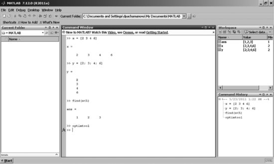
The standard MATLAB desktop window contains a Workspace window, a Command History window, and a Command window (see Figure 1). Depending on how you customize the MATLAB desktop window, however, you may see more or fewer windows. To check which windows are currently displayed and view other options, click on Desktop in the top MATLAB desktop window menu.

Figure 1 The Standard MATLAB Desktop

MATLAB commands are entered in the Command window. When a series of commands need to be given, it is more convenient to list them in an M-file, which is basically a file with instructions that MATLAB executes sequentially. Such files (scripts) are saved with the suffix “.m” and can be called from the prompt in the Command window typing their name (without the suffix “.m”). For example, if you create a file OptimizePortfolio.m with instructions on how to perform optimal portfolio allocation, you can call that file from the MATLAB command prompt by typing

>> OptimizePortfolio

(If the file is saved in a directory other than the default MATLAB directory, you will need to make sure that MATLAB can find the file. Select Desktop > Current Directory from the top menu and navigate to the correct directory before typing the command at the prompt.)

To create an M-file, you can use any text editing program, such as WordPad, NotePad, and the open source editor Emacs. In general, it is convenient to use an editor that recognizes the MATLAB file type and provides helpful highlighting for parts of the code that have different characteristics. (For example, comments in the code appear in different colors than commands.) MATLAB's own editor can do that, and Emacs can be set up to recognize the MATLAB file format as well.

To call MATLAB's editor in order to create or edit M-files, select Desktop > Editor from the top menu. Alternatively, you can use the shortcut buttons at the top of the MATLAB desktop window: the button to open a file that has already been created.

BASIC OPERATIONS AND MATRIX ARRAY CONSTRUCTION

Basic Mathematical Operations

MATLAB can perform many kinds of different mathematical operations, such as addition (+), multiplication (* or .*), square root (sqrt or sqrtm), and power (^). These commands can be entered at the command prompt. For example, typing

>> 3*sqrt(4) + 15

and pressing Enter produces the output

ans =
  21

To suppress output, use the semicolon (;). For example, entering

>> 3*sqrt(4) + 15;

does not result in any visible output in the command window. However, MATLAB still performs the calculation. To see this, let us assign the value of the above expression to a variable, ExpressionValue:

>> ExpressionValue = 3*sqrt(4) + 15;

Then, typing ExpressionValue at the command prompt, you get

>> ExpressionValue
ExpressionValue =
  21

Constructing Vectors and Matrices

As mentioned earlier, MATLAB's core data structures are vectors and matrices. For example, the command

>> x = [2 3 4 6]

produces a horizontal vector array (one row) x that contains the numbers 2, 3, 4, and 6.

The semicolon (;) is used to create new rows. To create a vertical vector array y with the same entries, you can enter

>> y = [2; 3; 4; 6]

or press Enter after entering each number. (MATLAB treats semicolons and carriage returns in array declarations as new lines.) The different syntax is useful depending on the source for downloading the data that populate the arrays.

Matrices are declared similarly. For example, a 2-by-2 matrix X can be specified as

MATLAB is case-sensitive; that is, it will treat the matrix X and the vector x defined earlier as separate variables.

Special commands exist for declaring types of matrices that are used often. For example,

produces a 3×3 identity matrix.

Similarly, the commands ones(n,m) and zeros(n,m) can be used to declare matrices that contain only 0s or 1s of the desired dimension (n x m), and diag(x) can be used to create a matrix that has a vector x as its diagonal elements, and 0s everywhere else.

You can also “stack” matrices and vectors. For example,

Basic Array Operations

To transpose an array A, use the command transpose(A) or A’. This operation converts a horizontal vector into a vertical one and vice versa, and flips the elements of a matrix that contains real numbers in its entries around the diagonal, keeping the diagonal entries the same.

For example,

To multiply two arrays, you can simply use the multiplication command *. Since the operation * performs a matrix multiplication, you need to make sure that the matrix dimensions agree. For example, an error results in the case when the 1×4 array x is multiplied by the 2×4 array X:

>> x*X
??? Error using ==> mtimes
Inner matrix dimensions must agree.

To multiply x and X correctly, you can instead type

If you need to perform an element-by-element multiplication of two arrays (of equal sizes), use the .* operator. For example,

Note that this is different from the matrix product. The matrix product would produce the following result:

When a matrix array is multiplied by a number, all of the array's entries are multiplied by that number. Similarly, if a number is added to a matrix array, the number will be added to all of the elements of the matrix. For example,

Extracting Information from Arrays

Suppose you have a matrix array Data with financial data on annual stock returns over 10 years for 1,000 companies traded on the New York Stock Exchange, and you would like to check the entry for the return on stock 253 in year 7. You are dealing with a 10x1000 matrix array in which each row is a time period and each column contains the returns on a particular stock. You are looking for the element in row 7, column 253 of this array. This can be requested with the command Data(7,253).

Suppose now that you would like to extract information on all of stock 253's returns over the 10 years. This means that you are looking for the elements of column 253 of the matrix array. This can be requested with the command Data(:,253). The colon operator replaces the row index to specify that elements with all indexes in the 253rd column should be produced. Similarly, if you would like to request all elements in the same row (e.g., the returns on all stocks in year 7), you can use the colon operator again: Data(7,:).

To illustrate the output, let us use the matrix array X. To find out what the value of the element in row 1, column 3 is, enter

>> X(1,3)
ans =
   3

The third column of X is

>> X(:,3)
ans =
   3
   7

Similarly, the second row of X can be obtained as

>> X(2,:)
ans =
   5  6  7  8

IMPORTANT MATLAB FUNCTIONS

MATLAB supports a number of built-in functions. A function is written as a command and takes arguments as inputs in parentheses. It processes the inputs by using operations hidden from the user and passes the final results back to the user. While we cannot cover many of the MATLAB functions in this brief introduction, we illustrate how functions work with an example of the function find, which can be useful in many situations.

Find takes in an array and a condition as arguments and returns the indexes of elements within the array that satisfy the condition. In addition to traditional applications, find can be very helpful when dealing with missing data, which happens often with financial time series.

Suppose you want to find the indexes of the elements that are less than 5 of the 1×4 array x from the previous section. At the prompt, type

>> find(x<5)

The result is

ans =
   1  2  3

Now let us see how find works when the array is a matrix rather than a vector. Recall that Y was the matrix array obtained by stacking x and X. Suppose you want to find the indexes of the elements in the array that are less than 5. At the prompt, type

>> ind = find(Y<5)

MATLAB creates the following array:

ind =
 1  
 2  
 4  
 5  
 7  
 8  
11 

MATLAB treated the matrix array as a stacked-up collection of column vectors. The elements of the array ind correspond to the indexes of the elements in that long column vector. Obtaining the actual elements of Y that correspond to these indexes can be accomplished by typing

>> Y(ind)

This produces the answer

ans =
   2 
   1 
   3 
   2 
   4 
   3 
   4	 

The indexing of an array as a sequence of stacked columns works well if the array is a vector, but it can get confusing if the array is a matrix. In the latter case, it is more intuitive to obtain the indexes as a row and column index. For example,

>> [indRow,indCol] = find(Y<5)

produces

indRow =
   1
   2
   1
   2
   1
   2
   2
indCol =
   1
   1
   2
   2
   3
   3
   4

This means that the following elements of Y have values less than 5: (row 1, column 1), (row 2, column 1), (row 1, column 2), and so on. Unfortunately, looking up the actual values of the elements of Y as Y(indRow,indCol) does not work.

CREATING USER-DEFINED FUNCTIONS

The compactness of the function syntax makes functions desirable when a user needs to call a certain sequence of commands often. For example, the Black-Scholes formula for pricing European options takes a number of steps to compute. It is convenient to have a function that returns one value—the option price—to the user after the user inputs values of factors that determine that price, such as the strike price, the time to maturity, the volatility, and so on.

Functions need to be written in M-files. Although general script M-files can contain any sequence of instructions that will be completed when the name of the file is typed at the MATLAB prompt, function M-files need to start with a specific first line. That line contains the word “function” and a declaration of the function name, inputs, and outputs. The function name and the name of the M-file should be the same.

The Black-Scholes formula already exists in the Financial Toolbox, so it is convenient to see how the price is computed and discuss important aspects of writing user-defined functions. (We have skipped some lines in the code for the sake of brevity.) Users can view the source code for some of the advanced MATLAB functions in the toolboxes by entering type function name at the prompt.

>> type blsprice
function [call,put] = blsprice(S, X, r, T, sig, q)
% BLSPRICE Black-Scholes put and call option pricing.
% Compute European put and call option prices using a Black-Scholes model.
%
% [Call,Put] = blsprice(Price, Strike, Rate, Time, Volatility)
% [Call,Put] = blsprice(Price, Strike, Rate, Time, Volatility, % Yield)
%
% Optional Input: Yield
%
% Inputs:
% Price - Current price of the underlying asset.
% Strike - Strike (i.e., exercise) price of the option.
% Rate - Annualized continuously compounded risk-free rate of
% return over the life of the option, expressed as a positive decimal number.
% Time - Time to expiration of the option, expressed in years.
% Volatility - Annualized asset price volatility (i.e., annualized
% standard deviation of the continuously compounded asset return),
% expressed as a positive decimal number.
% Optional Input: Yield - Annualized continuously compounded yield of the
% underlying asset over the life of the option, expressed as a decimal
% number. If Yield is empty or missing. the default value is zero. For
% example, this could represent the dividend yield (annual dividend rate
% expressed as a percentage of the price of the security) or foreign
% risk-free interest rate for options written on stock indices and
% currencies, respectively.
%
% Outputs:
% Call  - Price (i.e., value) of a European call option.
% Put   - Price (i.e., value) of a European put option.
…
%
…

% Copyright 1995-2005 The MathWorks, Inc.
% $Revision: 1.8.2.5 $ $Date: 2005/09/18 16:19:06 $

%
% Input argument checking & default assignment.
%

if nargin < 5
 error('Finance:blsprice:InsufficientInputs', …
   'Specify Price, Strike, Rate, Time, and Volatility.')
end

if (nargin < 6) ∥ isempty(q)
  q = zeros(size(S));
end

message = blscheck('blsprice', S, X, r, T, sig, q);
  error(message);
%
% Perform scalar expansion & guarantee conforming arrays.
%

try
 [S, X, r, T, sig, q] = finargsz('scalar', S, X, r, T, sig, q);
catch
 error('Finance:blsprice:InconsistentDimensions', …
 'Inputs must be scalars or conforming matrices.')
end

%
% Record array dimensions for output argument formatting.
%

[nRows, nCols] = size(S);

call = nan(nRows * nCols, 1);
put = nan(nRows * nCols, 1);

%
% Convert to column vectors for intermediate processing.
%

[S, X, r, T, sig, q] = deal(S(:), X(:), r(:), T(:), sig(:), q(:));

%
% Enforce some boundary conditions that produce warnings (e.g., logarithm
% of zero and divide by zero) and potential NaN's in the output option
% price arrays:
%
% (1) At expiration (i.e., T = 0), the price of all options is simply the
%   greater of their intrinsic value and zero.
%
% (2) When the price of the underlying asset is zero (i.e., S = 0), the value
%   of a call option is zero and the value of a put option is equal to its
%   present value of the strike price (X). This boundary condition enforces
%   the "absorbing barrier" property associated with the geometric Brownian
%   motion diffusion process governing the price path of the underlying
%   asset (S).
%
% (3) When the strike price is zero (i.e., X = 0), the value of a put option
%   is zero and the value of a call option is equal to the price of the
%   underlyer (S).
%

isTimeZero    = (T == 0); % Expired options.
call(isTimeZero) = max(S(isTimeZero) - X(isTimeZero), 0);
put (isTimeZero) = max(X(isTimeZero) - S(isTimeZero), 0);

isStockZero    = (S == 0);
call(isStockZero) = 0; % Worthless calls.
if any(isStockZero)
 put(isStockZero) = X(isStockZero) .* exp(-r(isStockZero).*T(isStockZero));
end
isStrikeZero    = (X == 0);
call(isStrikeZero) = S(isStrikeZero);
put (isStrikeZero) = 0; % Worthless puts.

%
% Suppress a divide by zero warning ONLY for zero volatility conditions. Other
% warnings could be valuable.
%

state = warning; % Store the current state.

if any(sig == 0)
  warning('off', 'MATLAB:divideByZero')
end
%
% Now apply the general Black-Scholes European option pricing formulae,
% excluding the boundary cases handled above, and explicitly handling
% calculations that produce 0/0 = NaN's for the parameters of the
% cumulative normal distribution function (i.e., d1 & d2).
%
% NaN's occur when S = X, r = q, and Sigma = 0. This situation corresponds to
% at-the-money options written on riskless underlying assets. Such assets
% should earn the risk-free rate less the dividend yield. But when r = q, the
% net growth rate is also zero, resulting in 0/0 = NaN.
%

i = ∼(isTimeZero | isStockZero | isStrikeZero);

d1 = log(S(i)./X(i)) + (r(i) - q(i) + sig(i).^2/2) .* T(i);
d1 = d1 ./(sig(i).*sqrt(T(i)));
d2 = d1 - (sig(i).*sqrt(T(i)));

d1(isnan(d1)) = 0;
d2(isnan(d2)) = 0;

call(i) = S(i) .* exp(-q(i).*T(i)) .* normcdf( d1) - …
 X(i) .* exp(-r(i).*T(i)) .* normcdf( d2);
put (i) = X(i) .* exp(-r(i).*T(i)) .* normcdf(-d2) - …
 S(i) .* exp(-q(i).*T(i)) .* normcdf(-d1);

warning(state) % Restore the state.

%
% Reshape the outputs for the user.
%

call = reshape(call, nRows, nCols);
put = reshape(put , nRows, nCols);
% [EOF]

Some aspects of this function are very complicated for a beginner, but a review of the function syntax helps create a list of useful pointers to which you can refer when creating your own functions:

• The first line contains the word function followed by a specification of the outputs of the function call (in this case, [call,put]). Note that a function can have more than one output. After calling the function, MATLAB computes the values for the outputs, and the variable call will contain the price of a European call option, while the variable put will contain the price of a European put option. Next, we have an equal sign followed by the name of the function (blsprice) and the arguments for the function (S for current stock price, X for strike price, r for rate of return, T for time to maturity, sig for volatility, as well as the optional argument yield for continuous dividend yield).
• When the function is called with specific input values, you can assign the output to variables. For example,

  >> [callOutput,putOutput]
  = blsprice(110,100,0.10,2,0.40)
  callOutput =
  38.1757
  putOutput =
  10.0488
  

• The names of the input variables need to participate in calculations in the function. For example, S appears as the current stock price in the first line (function [call,put] = blsprice(S, X, r, T, sig, q)), and this is the same variable that is used to store the value of the stock price in the computations. Similarly, the names of the output variables (call and put) should appear somewhere in the text of the function and be assigned an expression, which can then be returned to the user.
• Note the abundance of the percentage sign (%) in the function code. This sign is used for writing comments that are ignored by MATLAB when executing the code. It is always a good idea to comment abundantly in order to be able to retrace your reasoning later. The first comment line is called “the H1 line,” and it is the line that is searched by the MATLAB built-in function lookfor. Lookfor searches all MATLAB files containing a keyword in their first line. (This is useful if you are not sure which function to use for a specific purpose, and you would like to find the names of all functions that may be relevant.) Therefore, it is important to provide a meaningful description of your function in the first commented line. After the first line, you can continue with a more detailed description of the function and list references.

CONTROL FLOW STATEMENTS

M-files, whether of a generic or function kind, can contain more advanced operations than matrix manipulation. Next, we briefly review a couple of control flow statements that are often used in such files: the for loop and the if statement.

The general format of a for loop is

for n = array
commands
end

The commands inside the for loop are executed once for every value in the column in the array. (Typically, the array is a vector of numbers, so the loop is executed once for every number.) For example,

for n = 1:5
v(n) = sqrt(n);
end

results in

v =
   1.0000 1.4142 1.7321 2.0000 2.2361

The array 1:5 is equivalent to [1 2 3 4 5]. MATLAB starts out with n = 1, computes its square root, and assigns it to v(1). Then, it keeps repeating the process until it has computed v(5) for n = 5.

Loops in MATLAB are often necessary, but as a general rule MATLAB is more efficient in array operations than in loops. For example, the same effect (adding 10 to each element of the vector x) can be achieved in two ways:

for n = 1:4
x(n) = x(n) + 10;
end

and

>> x = x+10

Both of them result in

x =
  12 13 14 16

The second command would typically be completed faster. Loops are not as inefficient as they used to be in older versions of MATLAB, however—the difference in speed between the two approaches has been greatly reduced in the latest versions of the software.

The if statement has the following general format:

if expression
commands
end

The commands are completed only if all elements in the expression are true. A somewhat more complex if statement is

if expression1
commands1
elseif expression2
commands2
else expression3
commands3
end

Commands1 are completed if expression1 is true. If expression1 is not true, MATLAB moves on and checks if expression2 is true. If expression2 is true, commands2 are completed. If expression2 is not true either, MATLAB moves to expression3. If expression2 is true, commands3 are completed; otherwise MATLAB exits. The elseif or else commands are optional in if statements.

There are several other useful control flow statements, such as the while loop, switch-case constructions, and try-catch blocks. See the MATLAB manual and help for more detail.

GRAPHS

MATLAB is well known for its beautiful graphing capabilities. The most common function for plotting two-dimensional (2-D) graphs is plot.

To illustrate how plot works, suppose we would like to plot the standard normal probability distribution. We will use the function normpdf (available from the Statistics Toolbox), which computes the probability density function (PDF) of a normal random variable.

The command

>> x = linspace(-6,6,100)

creates a vector x with 100 values, equally spaced between the minimum value −6 and the maximum value +6. (In reality, the normal distribution stretches from negative infinity to positive infinity, but it is highly unlikely that we will obtain realizations that are greater than 6 standard deviations away from the mean of 0, so we focus on plotting the center of the distribution.)

The command

>> y = normpdf(x)

computes the values of the normal probability distribution function for every value in the array for x.

To plot x versus y, use

>> plot(x,y)

The result is the graph in Figure 2.

Figure 2 A Plot of the PDF of the Normal Distribution

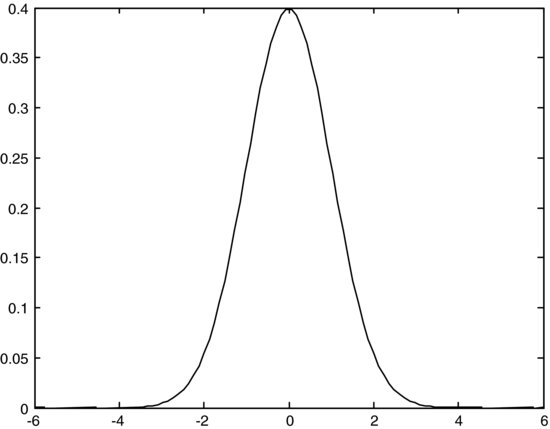
Figure 3 A Plot of the PDF of the Normal Distribution (with Modified Options)

You can play with the options for the graph. For example,

>> plot(x,y,'r:p'), title('Normal PDF'),
     xlabel('x'), ylabel('pdf')

plots the same graph as a red dotted line with a pentagram symbol, labels the horizontal (x) and the vertical (y) axes, and creates a title for the graph (see Figure 3).

To plot multiple graphs on the same picture, use the command hold on before you start and hold off when you are done with the instructions. For example, suppose we would like to plot the standard normal distribution and a standard t-distribution with 5 degrees of freedom on the same graph in order to compare them. The following sequence of commands accomplishes this.

First, we declare a variable that follows a t-distribution with 5 degrees of freedom:

Figure 4 Illustration of hold on / hold off Effect

>> t=tpdf(x,5);

Then, we plot the graph:

>> hold on
>> plot(x,y,'r:p'), xlabel('x'),
     ylabel('pdf')
>> plot(x,t);
>> title('Normal Versus T Distribution'),
>> hold off

The results are displayed in Figure 4.

Alternatively, you can list several pairs of variables inside the plot function. For example,

>> plot(x,y,'r:p',x,t); xlabel('x'),
 ylabel('pdf')
>> legend('Normal PDF','T PDF')
>> title('Normal Versus T Distribution
 with 5 DoF'),

This script also creates a legend (Figure 5).

Figure 5 Changing Defaults and Plotting Multiple Graphs with the plot Function

Legend, titles, and other graph attributes can be added and modified also after the basic plot command has been given and a graph window has popped up. To modify an existing graph's options, click on the corresponding items in the top menu of the graph window.

Suppose now that we would like to plot the two PDFs side by side in the same figure. To graph several separate graphs in the same figure, use the command subplot(number of rows, number of columns, index of graph within the graph array).

For example, the code

>> subplot(1,2,1), plot(x,y,'r:p'),
  xlabel('x'), ylabel('pdf')
>> title('(a) Normal PDF')
>> subplot(1,2,2), plot(x,t);
  xlabel('x'), ylabel('pdf')
>> title('(b) T PDF')

produces the graph in Figure 6.

Figure 6 Multiple Plots within the Same Figure

Finally, we briefly discuss three-dimensional (3-D) graphs. They can be created with commands like plot3 and surf, and as a general matter are more complex.

The command plot3(first variable x, second variable y, third variable z) plots points in 3-D space whose three coordinates are given by the vectors or matrices (x,y,z) in the three arguments of the function. The arguments need to be arrays of equal sizes.

The command surf(x, y, z) plots a shaded surface using z as the height and (x, y) as the vectors or matrices that define the other two dimensions of the surface. When x and y are vector arrays, as is the case in most financial applications, the number of rows for z should be the length of the vector array y, and the number of columns for z should be the length of the vector array x.

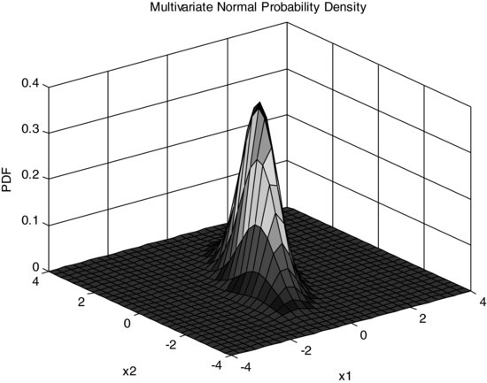
For example, suppose we would like to plot a multivariate normal distribution function for two normal variables, x1 and x2, that have means of 0 and are correlated with covariance matrix [0.25 0.3; 0.3 1]. (Note that this notation means that the variance of x1 is 0.25 (the standard deviation of x1 is 0.5), the variance of x2 is 1 (the standard deviation of x2 is 1), and the covariance of x1 and x2 is 0.3.

The multivariate normal distribution function can be computed with the MATLAB function mvnpdf(X,mu,Sigma). The arguments mu and Sigma are the vector array of average (expected) values for the normal random variables and their covariance matrix, respectively. In this case, we have two normal random variables, so mu=[0 0] and Sigma = [0.25 0.3; 0.3 1]. The first argument in the function (matrix X) provides the points at which the function should be evaluated. The function is evaluated for every row of X, taking the elements in that row as the coordinates of the point at which the function should be evaluated. Therefore, since in our example we are looking at two normal random variables, there should be two columns of the matrix X. We cannot simply provide two columns with, say, equally spaced values for x1 and x2. If we do, MATLAB would pair each entry of x1 with the corresponding entry of x2, and will only use those combinations of coordinates, so the plot will look two-dimensional. The columns of X should provide a grid. In other words, we cannot simply provide possible coordinates along each axis and expect that MATLAB will know to take every combination of possible coordinates to obtain the points at which to plot the function. To create this grid of points, we need to go through a couple of steps.

First, we would use the function [X1,X2] = meshgrid(x1,x2). It creates two matrices. The number of rows in the first matrix, X1, is the same as the number of elements in the vector y (i.e., the number of rows equals length(y), another useful MATLAB command). Each row of the column X1 contains identical entries: the entries of the vector x. The matrix X2 contains the same number of columns as the number of elements in the vector x, and each column contains an identical copy of the vector y. While perhaps difficult to imagine at first, X1(i,j) and X2(i,j) cover all possible combinations of the elements of the original vectors, x and y.

The second step is to create the array [X1(:), X2(:)]. The colon operator (:) has multiple uses, but in the context of being used as an argument for a matrix, it takes all entries of a matrix, column by column, and lists them as a vector array. Therefore, the array [X1(:),X2(:)] would contain two columns with every possible combination of coordinates generated by the original list in the vector arrays x and y.

To summarize, here are the commands used to generate 30 points between –4 and 4 along each coordinate x1 and x2, then to evaluate the multivariate normal PDF at each combination of coordinates:

>> x1 = linspace(-4,4,30);
  x2 = linspace(-4,4,30);
>> Sigma = [0.25 0.3; 0.3 1]; mu = [0 0];
>> [X1,X2] = meshgrid(x1,x2);
>> z = mvnpdf([X1(:),X2(:)],mu,Sigma);

The output of this sequence of commands is a vertical array of values that represent the multivariate normal PDF evaluated at each combination of coordinates. (If you skip the semicolon at the end of the last row with the function mvnpdf, you can see what the output looks like. You can also use the command size(z) to check the dimensions of z.) Now we would like to plot these values. We will use the surf function.

Figure 7 Three-Dimensional Plot of a Multivariate Normal Distribution

The surf function's third argument, z, needs to be a matrix whose entries represent the values of the function to be plotted at each combination of coordinates. However, we obtained a vector of values for the PDF. We need to “reshape” that vector back into a matrix. This can be done with the command Z = reshape(z,m,n). The function reshape takes the array z and goes through the elements of z columnwise. The first m elements of z become the first column of the new matrix Z, the next m elements of z become the second column of the matrix Z, and so forth until n columns for Z are created. In this example, we would like to create length(x1) columns and length(x2) rows. (This may be a bit confusing, but, as we mentioned earlier, the function surf expects the third argument to be a matrix with the number of columns equal to the size of the first argument, and the number of rows equal to the size of the second argument.)

>> Z = reshape(z,length(x2),length(x1));
>> surf(x1,x2,Z);
>> title('Multivariate Normal
  Probability Density')
>> axis([-4 4 -4 4 0 0.4]);
>> xlabel('x1'), ylabel('x2'),
  zlabel('PDF'),

The resulting graph is in Figure 7.

IMPORTING DATA AND INTERACTING WITH SPREADSHEETS

MATLAB recognizes files with the extension .dat as data files. Such files should contain text structured in rows and columns. For example, suppose that the file returns.dat contains daily annual returns on the stocks traded in the NYSE for 10 years. The command

>> load returns.dat

imports the data in the file into a data structure—a matrix array with rows and columns that can then be referenced using some of the commands we described earlier.

Many financial companies build their infra-structure around Microsoft Excel. The MATLAB core product contains some useful functions for importing Excel data and exporting MATLAB results to spreadsheets. The function

>> xlsread(‘fileName’,'sheetName’,
 ’range’)

allows the user to read into MATLAB the data stored in file fileName, worksheet sheetName, cells in range range. Instead of a range in the spreadsheet, you can state an array name if you had named the array of cells in advance. Variations of this command exist; for instance

>> xlsread(‘fileName’,-1)

allows the user to select the range in fileName directly, through interactive selection in Excel. Type help xlsread at the MATLAB command prompt for further information.

The function

>> xlswrite(‘fileName’,output,'sheetName’,
 ’cell’)

allows the user to export MATLAB results (output) to a worksheet (sheetName) in an Excel file (fileName). MATLAB preserves the dimensions of the output and writes it to the spreadsheet starting at cell reference cell. For example, if output is a horizontal array of numbers, MATLAB will write the data in a row in the Excel file, starting at cell.

MATLAB operations work within the xlswrite command. For example, you can switch the array dimensions (transpose) the output by using output’ inside the parentheses of the xlswrite command if you desire different output formatting in the Excel spreadsheet.

More sophisticated capabilities exist through MATLAB's Excel Link. With Excel Link, you can call MATLAB's functions directly from within Excel, thus ensuring access to MATLAB's superior computational and graphical capabilities. Excel Link is purchased as a separate toolbox. It can then be made visible from within Excel by selecting it as one of Excel's Add-Ins. There are 11 commands (they all start with “ML”) that allow for communicating data back and forth between Excel and MATLAB. For example, =MLAppendMatrix() creates or appends a matrix in MATLAB with data from an Excel spreadsheet.

A word of caution: Excel Link formulas are not case sensitive. For example, MLAppendMatrix and mlappendmatrix are the same. However, MATLAB functions and variables called through these links are case sensitive. For example, x and X would still be treated as two separate variables.

EXAMPLES

This section discusses several scripts and functions in MATLAB that can be used in financial applications. The goal is to illustrate the use of toolboxes in MATLAB and to provide concrete examples of some of the tools introduced earlier in the entry.

Table 1 MATLAB Optimization Toolbox Functions/Solvers Appropriate for Specific Types of Optimization Problems

Optimization in MATLAB

Optimization is an area in applied mathematics that, most generally, deals with efficient algorithms for finding an optimal solution among a set of solutions that satisfy given constraints. The first application of optimization in finance was suggested by Harry Markowitz in 1952, in a seminal paper that outlined his mean-variance optimization framework for optimal asset allocation. Some other classical problems in finance that can be solved by optimization algorithms include:

MATLAB's Optimization Toolbox contains solvers for a range of optimization problems. MATLAB expects optimization formulations to be passed to its solvers in an array form and has functions that call specific solvers for specific types of optimization problems. (See Table 1 for a quick overview. See also MATLAB's help for a complete listing.) If the Global Optimization Toolbox is available, the range of solvers is expanded to include randomized search algorithms.

The most often used solver in MATLAB is fmincon, which is the solver for general nonlinear optimization. However, if you know the type of problem you are trying to solve, you are always better off giving the optimization software as much information as you can in order to make the optimization process more accurate and efficient. In financial applications, you are most likely to encounter situations in which you need linprog (a linear programming solver), quadprog (a quadratic programming solver), bintprog (a binary programming solver), and randomized search algorithms, such as simulannealbnd and ga.

We will use linprog and quadprog to solve two examples of portfolio allocation problems. Before we show the actual implementation, we need to explain how solvers are actually called in MATLAB. There are two ways to call the solvers: as functions directly from the command prompt (equivalently, from within M-files), or through the optimization tool.

The MATLAB optimization tool provides an interface between the solvers and the user. While using such an interface may not be optimal when solving sequences of optimization problems, as in the case of dynamic programming or stochastic programming, it is quite convenient when solving a single optimization problem, because it lists all available solvers, prompts the user for the different inputs that the optimization solvers expect, and allows for easy manipulation of the options. Options can be specified directly when a solver is called from the command prompt as well, but that is more difficult for MATLAB beginners.

The optimization tool is called by typing optimtool at the MATLAB command prompt. The optimization tool dialog box is shown in Figure 8. The panel on the left-hand side is dedicated to the specification of the inputs: the type of solver that needs to be called, the arrays with the problem data, the starting point, and so on. The panel in the middle allows for changing the level of tolerance in the search for the optimal solution. For example, the Function tolerance is currently set at the default value of 1e-06, which is 10-6. This means that the selected algorithm will continue to iterate through solutions until the improvement in successive objective function values becomes smaller than 10-6. Sometimes, such level of accuracy is unnecessary. For example, if our objective function is measured in dollars and cents (e.g., we are maximizing dollar return as in the simple portfolio allocation example we will discuss next), then technically we do not need precision beyond 2–3 digits after the decimal point. Therefore, we can speed up the algorithm by relaxing the requirements on tolerance. Other useful options include level of display (whether to show iterations of the optimization algorithm or not) and function plots at intermediate stages.

Figure 8 The Optimization Tool Interface in MATLAB

Linear Optimization: Simple Portfolio Allocation

Let us consider a specific example to illustrate the use of the optimization function linprog. (For more details, see section 5.3.1 in Pachamanova and Fabozzi, 2010.)

The portfolio manager at a large university in the United States is tasked with investing a $10 million donation to the university endowment. He has decided to invest these funds only in mutual funds and is considering the following four: an aggressive growth fund (Fund 1), an index fund (Fund 2), a corporate bond fund (Fund 3), and a money market fund (Fund 4), each with a different expected annual return and risk level. (The risk level measurement is deliberately simplified for the sake of this example.) The investment guidelines established by the Board of Trustees limit the percentage of the money that can be allocated to any single type of investment to 40% of the total amount. The data for the portfolio manager's task are provided in Table 2. In addition, in order to contain the risk of the investment to an acceptable level, the amount of money allocated to the aggressive growth and the corporate bond funds cannot exceed 60% of the portfolio, and the aggregate average risk level of the portfolio cannot exceed 2. What is the optimal portfolio allocation for achieving the maximum expected return at the end of the year, if no short selling is allowed?

Table 2 Data for the Portfolio Manager's Problem

The vector of decision variables for this optimization problem can be defined as x=(x1, x2, x3, x4): amounts (in $) invested in Fund 1, 2, 3, and 4, respectively.

Let the vector of expected returns be μ = (20.69% ,5.87% ,10.52% ,2.43%). Then, the objective function can be written as

It represents the optimal expected dollar amount at the end of the year.

There are also several constraints.

4*(proportion of investment with risk level 4) + 2*(proportion of investment with risk level 2) + 1*(proportion of investment with risk level 1) ≤ 1 or, mathematically,

In this particular example we know that the total amount x1+x2+x3+x4=10, 000, 000, so the constraint can be formulated as

1. The maximum investment in each fund cannot be more than 40% of the total amount ($4,000,000). These constraints can be written as

2. Given the no short selling requirement, the amounts invested in each fund cannot be negative. These are nonnegativity constraints: .

The final optimization formulation can be written in matrix form. The objective function is

Let us organize the constraints into groups according to their signs. This will be useful when we input the constraints into MATLAB.

This is a linear optimization problem because all constraints and the objective function are linear. To solve linear optimization problems with MATLAB, use linprog (f,A,b,Aeq, beq,lb,ub). The function arguments f,A,b, Aeq,beq,lb,ub correspond to the following LP formulation:

Therefore, before calling linprog, you need to write the problem formulation in this particular form. We include the complete MATLAB script below.

1 numAssets = 4;
2 expReturnsVec = [0.2069 0.0587 0.1052 0.0243]';
3 %create placeholders for an array of decision variables
4 %(amounts to invest in
5 %each fund) and the optimal portfolio expected return (to be filled out
6 %after the optimization)
7 
8 amountsVec = zeros(numAssets,1);
9 optReturn = [];
10
11 %vector of coefficients of objective function f since MATLAB expects
12 %minimization (and we are maximizing), take the negative of the function
13 %we are trying to maximize
14 f = -expReturnsVec;
15
16 %A, matrix of coefficients in constraints with inequalities so that
17 %Ax<=b 
18 A = [1 0 1 0;
19   4 2 2 1;
20   1 0 0 0;
21   0 1 0 0;
22   0 0 1 0;
23   0 0 0 1];
24
25 %b
26 b = [6000000 20000000 4000000 4000000 4000000 4000000]';
27
28 %Aeq, matrix of coefficients in constraints with equalities so that
29 %Aeq*x=beq
30 Aeq = ones(1,numAssets);
31
32 %beq
33 beq = 10000000;
34
35 %lower bounds: nonnegativity requires that all decision variables are >= 0
36 lb = zeros(numAssets,1);
37
38 %upper bounds can be left infinite (although, technically, we cannot invest
39 %more than the $10m we have available)
40 ub = inf*ones(numAssets,1);
41 
42 [amountsVec,optReturn] = linprog(f,A,b,Aeq,beq,lb,ub);
43 
44 format('bank'),
45
46 amountsVec
47 %revert to correct number for maximum return (reverse sign)
48 optReturn = -optReturn

The process for formulating the optimization problem is as follows. First, we ask ourselves what corresponds to the vector of decision variables x in the linprog formulation. In our example, x maps directly to the vector of amounts to invest in each asset. We then enter problem data, such as the expected returns vector expReturnsVec. We allocate empty arrays to store the values of the optimal solution amountsVec and the optimal value of the objective function optReturn after collecting the information from the solver.

Next, we create the input data for the linprog solver. The solver expects a vector of objective function coefficients f, which in our case is the vector of expected returns on the different assets. Note, however (line 14), that we specify f as -expReturnsVec. This is because MATLAB expects a minimization problem, and our objective function is to maximize expected revenue, so we need to convert our problem to the required form by minimizing the negative of the expression for the maximization objective. At the end (line 48), we take the negative of the optimal value for expected return found by the solver, so that we arrive at the actual optimal value for the maximization problem. The optimal values of the decision variables, which in this case are the amounts to invest, amountsVec, do not need to be modified after the optimization results are returned by the solver.

Lines 14–40 contain the specification of the other inputs in the problem. Note that we are in fact using the matrices of coefficients for the groups of constraints (inequality, equality, and nonnegativity) that we defined earlier. Namely, A (lines 18–23) is the matrix of left-hand-side inequality constraint coefficients; Aeq (line 30) is the matrix of left-hand-side equality constraint coefficients; b (line 26) is the vector of right-hand-side coefficients of the inequality constraints; and beq (line 33) is the vector of right-hand-side coefficients of the equality constraints (in our example, we have only one equality constraint). The lower bounds, lb (line 36), are the zeros from the right-hand-side of the nonnegativity constraints on the decision variables, so we create a vector array with size equal to the number of decision variables that contains only zeros. We have explicit upper bounds of $4,000,000 on each decision variable since we cannot invest more than that amount in each individual fund, so we could have stated those bounds as the input vector ub. However, these bounds have already been included in the matrix A, so we do not need to state them again. Instead, we state the individual upper bounds as infinity, that is, as the product of the number inf (in MATLAB, that denotes infinity) and a vector of ones. (See line 40 of the code.)

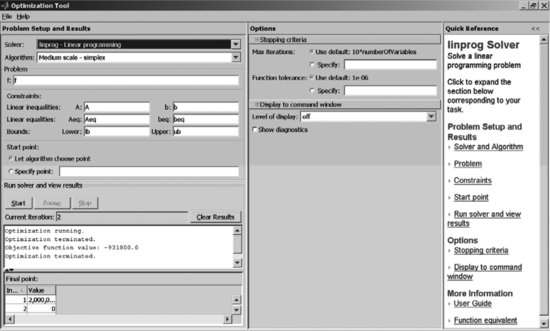
Figure 9 The Optimization Tool Dialog Box for the Portfolio Allocation Problem

An equivalent formulation of the constraints from MATLAB's perspective would have been to specify the arrays A, beq, and ub as

A = [1 0 1 0;
  4 2 2 1]
b = [6000000 20000000]’
ub = 4000000*ones(numAssets,1)

with all other input arrays remaining the same.

After all inputs have been specified, the linprog solver is called (line 42). The syntax in line 42 outputs requests that the output from the optimization be stored in the arrays we specified at the beginning, amountsVec and optReturn. The results are then printed to the screen and are formatted according to format(‘bank’) (line 44), which basically rounds numbers to two decimal places.

After running the M-file, we obtain the following output:

amountsVec =
 2000000.00
    0.00
 4000000.00
 4000000.00
optReturn =
   931800.00

If you prefer to solve the problem by using the optimization tool for solving this problem, you need to fill out the dialog box as shown in Figure 9. Select linprog as the solver from the drop-down menu at the top. Under Algorithm, you can either leave the default (Large Scale), or select Medium scale – simplex, which is appropriate because our problem is quite small. We entered the names of the arrays that correspond to the objective function coefficients and the constraint coefficients in the corresponding fields in the left panel of the dialog box. Note that these arrays must be prefilled; that is, they must be entered from the command prompt or read from a file before the problem is solved through the optimization tool; otherwise the solver will complain that these arrays are empty. You can make sure that the arrays f,A,b,Aeq,beq,lb,ub are filled in by checking first whether they are listed in the Workspace window at the upper left corner of the MATLAB desktop. Once all the input data are specified, click on the Start button in the left panel to solve the problem. The solution appears in the field below the Start button.

Figure 10 Handling the Structure of Optimization Results Exported from MATLAB's Optimization Tool

The optimization model can be saved as a script in an M-file by selecting File | Generate M-file from the main menu in the optimization tool. In addition, the optimization results can be exported to the workspace and further manipulated by selecting File | Export to Workspace. To export only the results, as opposed to the entire model, check Export results to a MATLAB structure named: optimresults. This creates a structure of results, optimresults, that shows up in the Workspace. So, for example, the optimal solution (the portfolio allocation) can be read by typing optimresults.x at the command prompt. (See Figure 10.) Similarly, the optimal value of the objective function can be retrieved by typing optimresults.fval at the command prompt.

Quadratic Optimization: Mean-Variance Portfolio Allocation

The classical mean-variance portfolio optimization problem as introduced by Harry Markowitz (1952) is to minimize the variance of portfolio return subject to the constraint that the expected portfolio return is at a certain level. Let us consider a slight variation of the problem, in which we require that the expected return is at least at a certain level rtarget. The mathematical formulation is

where w is the vector of portfolio weights (to be determined), μ is the vector of expected returns, Σ is the covariance matrix of returns, and ι is a vector of ones of appropriate dimension.

The minimum variance portfolio allocation problem is a quadratic optimization problem with linear constraints. The quadprog function in MATLAB solves exactly problems of this kind:

and is called with the command quadprog (H, f, A, b, Aeq, beq, lb, ub).

It is easy to see how to match the two formulations:

• x = w
• f = 0
• H = 2 Σ
• A = −μ’
• b = −rtarget
• Aeq = ι’
• beq = 1
• lb = −infinity
• ub = infinity

For example, the inequality constraint

in the mean-variance formulation is mapped to the inequality constraint assumed by the quadprog function

by rewriting the mean-variance constraint as

and setting A = −μ’ and b = −rtarget.

Suppose we are given a portfolio with a number of stocks equal to numAssets, expected returns for the stocks stored in a vertical vector muVec, covariance matrix SigmaMx, and required expected return of targetReturn. Consider a simple portfolio of two stocks with expected returns of 9.1% and 12.1%, standard deviations of returns of 16.5% and 15.8%, and a correlation of –0.22 (covariance of –57.35). A MATLAB script that uses input data for the two stocks, calls the optimization solver for several instances of the problem with different values of targetReturn, and plots the efficient frontier looks as follows:

numAssets = 2;
muVec = [9.1; 12.1];
SigmaMx = [272.25, -57.35;
 -57.35, 249.64];

targetReturn = 11;

%SINGLE OPTIMIZATION

%create the matrix X
H = 2*SigmaMx;

%create a vector of length numAssets with zeros
f = zeros(numAssets,1);

%create right hand and left hand side of inequality constraints
A = -transpose(muVec);
b = -targetReturn;

%create lower bounds array for asset weights (negative infinity)
lb = -inf*ones(numAssets,1);

%create upper bounds array for asset weights (infinity)
ub = inf*ones(numAssets,1);

%create right hand and left hand side of equality constraints
beq = [1];
Aeq = transpose(ones(numAssets,1));
[weights,variance] = quadprog(H,f,A,b,Aeq,beq,lb,ub);

%print results to screen
stdDev = sqrt(variance)
weights

%EFFICIENT FRONTIER
%loop through different values of the target portfolio returns, compute the
%optimal portfolio standard deviation, and plot the efficient frontier

iCounter = 1;

for iTRet = 9.5:0.5:12
 b = -iTRet;
 [weights,variance] = quadprog(H,f,A,b,Aeq,beq,lb,ub);
 y(iCounter) = iTRet;
 x(iCounter) = sqrt(variance);
 iCounter = iCounter + 1;
end

%plot efficient frontier
plot(x,y);
xlabel('Portfolio standard deviation'),
ylabel('Portfolio expected return'),
title('Efficient Frontier'),

The command

[weights,variance] = quadprog(H,f,A,b,
Aeq,beq,lb,ub);

ensures that the optimal solution to the optimization problem is stored in a vector called weights, and the optimal objective function value (the minimum portfolio variance) is stored in the scalar variance. This is an example of using a MATLAB built-in function. The portfolio standard deviation is computed as the square root of variance.

The MATLAB output from running the code above is as follows:

stdDev =
 10.4928
weights =
 0.3667
 0.6333

The script also contains an example of a for loop that runs the optimization problem for values of the target return between 9.5 and 12, increasing the target return by 0.5 at each iteration. The expected portfolio return and the optimal standard deviation obtained from the optimization output are stored in vectors x and y. The last few lines in the code plot the efficient frontier using the values stored in x and y, and label the graph.

Pricing a European Call Option by Simulation

Simulation is a technique for replicating uncertain processes and evaluating decisions under uncertain conditions. In the financial context, it typically involves generation of random numbers from particular probability distributions, using those for approximating the behavior of exogenous variables such as stock returns, and assessing outcomes of interest, such as the performance of a portfolio or the price of a financial instrument.

Through the Statistics Toolbox, MATLAB provides commands for generating the most commonly used random numbers directly. For example, a normal random variable can be simulated with

>> normrnd(mean,stdev,numRows,
 numColumns)

In the expression above, mean and stdev are the mean and the standard deviation of the normal random variable. numRows and numColumns specify the dimension of the array of random numbers we would like to generate.

We show how to use MATLAB's Statistics Toolbox to compute the price of a European call option with simulation under the assumptions that there are no transaction costs or market frictions, and the price of the underlying follows geometric Brownian motion. (The closed-form formula for pricing the option under these assumptions is the Black-Scholes formula.) Option pricing by simulation was first suggested by Boyle (1977). For further details on the implementation and more examples, see Pachamanova and Fabozzi (2010).

The evolution of the asset price at time t, St, can be described by the equation

where Wt is standard Brownian motion and μ and σ are the drift and the volatility of the process, respectively. For technical reasons (absence of arbitrage), when pricing an option, the drift μ is replaced by the risk-free rate r.

Under the assumption for the random process followed by the asset price, the value of the asset price ST at time T given the asset price St at time t can be computed as

where is a standard normal random variable. (If the stock pays a continuously compounded dividend yield of q, then we use (r – q – 0.5·σ2) instead of (r – 0.5·σ2) as the drift term.)

The price of the option can be approximated by creating scenarios for the stock price ST at time T, computing the discounted payoffs of the option, and finding the expected payoff of the option. Suppose we generate N scenarios for : (1),…, (N). Then, the price of a European call option with strike price K will be

The expression above is the expected value of the option payoffs; that is, the weighted average of the option payoffs. The “weight,” or the probability of each scenario, is 1/N.

In MATLAB, we create a function EuropeanCall (stored in a file EuropeanCall.m), which follows.

function CEPrice = EuropeanCall(initPrice,K,r,T,sigma,q,numPaths)
%function for evaluating the price of a European call option using crude
%Monte Carlo
%initPrice is the initial price, K is the strike price, r is the annual interest
%rate, T is the time to maturity, sigma is the annual volatility, q is the
%continuous dividend yield, numPaths is the number of scenarios to generate for
%the evaluation

CEpayoffs = zeros(numPaths,1);

%compute a vector array of asset prices, one for each scenario
assetPrices = initPrice*exp((r-q-0.5*sigma^2)*T+sigma*sqrt(T)*
normrnd(zeros(1,numPaths),ones(1,numPaths)));

CEpayoffs = exp(-r*T)*max(assetPrices - K,0);

CEPrice = mean(CEpayoffs);

In the function, we generate the (random) end points of numPaths paths for the underlying stock price under the assumption that the price follows geometric Brownian motion. We use the Statistics Toolbox function normrnd(mu,sigma), which in this case returns a vector array with the realizations of normal random variables. The array has the dimension of the mu and sigma vectors, which are vectors of zeros and ones, respectively, with length numPaths. Then, we generate a vector array of asset prices by calculating the asset price in each scenario. We use a nice feature in MATLAB, which is that we can pass an array (namely, normrnd(zeros(1,numPaths), ones(1,numPaths)) into a formula (namely, initPrice*exp((rq-0.5*sigma^2)*T + sigma*sqrt(T)* normrnd(zeros(1, numPaths),ones(1,numPaths))), and MATLAB automatically creates an array with results (assetPrices). In other programming languages, we would need to implement this by creating a for loop.

Finally, we calculate the option price CEPrice as the average of the payoffs of the option in each scenario by using the function mean.

Pricing a European Call Option Using a Sobol Sequence

In the function EuropeanCall, we used the MATLAB built-in function normrnd from the Statistics Toolbox with arguments that were arrays of zeros and ones to generate a set of realizations drawn from a standard normal probability distribution and compute a set of paths for the price of the underlying. Alternatively, we could have generated a set of quasirandom numbers that sometimes lead to a faster and more accurate estimation for the option price. (See the discussion in Chapter 14 of Pachamanova and Fabozzi, 2010; Chapter 6 in McLeish, 2005; or section 5.2.3 of Chapter 5 in Glasserman, 2004.) MATLAB's Statistics Toolbox contains built-in syntax for computing the elements of some low-discrepancy sequences, such as the Sobol sequence (Sobol, 1967). Namely, the function sobolset(d) computes a Sobol sequence of dimension d, and the sequence can then be retrieved with the command net. For example,

seq = sobolset(3); net(seq,5)

returns the first five elements of a Sobol sequence of dimension 3.

The calculation of the European call option price using the Sobol sequence is shown in the function EuropeanCallSobol below.

function SCEPrice = EuropeanCallSobol(initPrice,K,r,T,sigma,q,numPaths)
%function for evaluating the price of a European option using
%a Sobol sequence
%initPrice is the initial price, K is the strike price
%r is the annual interest rate, T is the time to maturity, sigma is the
%annual volatility
%q is the continuous dividend yield
%numPaths is the maximum number of scenarios to generate for the evaluation

SCEpayoffs = zeros(numPaths,1);
%use the sobolset function in the Statistics Toolbox to generate the
%sequence
seq = sobolset(1);
SobolPoints = net(seq,numPaths+1);
%drop the first element, which is 0
SobolPoints = SobolPoints(2:numPaths+1);

%compute a vector array of asset prices, one for each Sobol point
assetPrices = initPrice*exp((r-q-0.5*sigma^2)*T+sigma*sqrt(T)*
norminv(SobolPoints));

%compute a vector array of discounted payoffs, one for each scenario 
%generated from a Sobol point

SCEpayoffs = exp(-r*T)*max(assetPrices - K,0);

%compute price of option
SCEPrice = mean(SCEpayoffs);

Again, in this function, we passed an array (SobolPoints) into a formula (initPrice *exp((rq-0.5*sigma^2)*T + sigma*sqrt(T)*norminv(Sobol-Points))), and MATLAB automatically created an array with results (assetPrices).

The Sobol sequence generated in the function is of dimension 1 and length numPaths+1. We created it with the commands

seq = sobolset(1);
SobolPoints = net(seq,numPaths+1);

and remove the first element, which is 0, with the command

SobolPoints = SobolPoints(2:numPaths+1);

(As explained in Chapter 14 of Pachamanova and Fabozzi [2010], it is common to drop some number of elements of low-discrepancy sequences. It takes a certain “warming up” for the low-discrepancy sequence to begin producing stable and accurate estimates.)

Computing the Black-Scholes Price of a European Option Using the Financial Toolbox

The price for the European option obtained in the ways described in the previous two sections is, of course, an approximation. It will vary slightly depending on the specific set of scenarios simulated with the normrnd function, or on the number of points generated with the Sobol sequence. The true option price under the stated assumptions is given by the Black-Scholes formula. (See Black and Scholes, 1973; Hull, 2008; or Pachamanova and Fabozzi, 2010.) As we mentioned earlier in this entry, the function blsprice in MATLAB's Financial Toolbox can compute this price. For example, for an initial price of 100, a strike price of 110, an interest rate of 6%, time to maturity of 1 year, and volatility 40%, the Black-Scholes price for the European call option will be computed by typing

>> blsprice(100, 110, 0.06, 1, 0.40)

at the MATLAB prompt. MATLAB returns

ans =
 14.4018

You should get a similar price by typing the names of the user-defined functions we wrote previously,

>> EuropeanCall(100,110,0.06,1,0.40,
  0,20,1000)

to compute it with simulation, or

>> EuropeanCallSobol(100,110,0.06,1,
  0.40,0,1000)

to compute it by using a Sobol sequence. Here we are requesting that the price be evaluated with 1,000 paths for the price of the underlying. The greater the number of paths, the closer the estimates will be to the Black-Scholes price. For this example, we obtained 14.3772 for the option price by crude Monte Carlo simulation, and 14.0882 by using the Sobol low-discrepancy sequence. The variability for the option price estimated using the crude Monte Carlo simulation approach is large, so readers can expect answers that differ quite a bit.

KEY POINTS

• MATLAB uses a number-array-oriented programming language; that is, a programming language in which vectors and matrices are the basic data structures.
• Array operations are very efficient in MATLAB.
• Specialized MATLAB toolboxes provide additional capabilities, save time, and simplify model building. Some toolboxes build on the capabilities of other toolboxes and need to be purchased in groups.
• An M-file is a file with instructions that MATLAB executes sequentially. Such files are saved with the suffix “.m” and can be called from the prompt in MATLAB's Command window by typing their name without the suffix “.m”.
• M-files can be scripts, that is, a simple listing of instructions for MATLAB, or functions, which take in a certain number of arguments and return a certain number of outputs.
• While general script M-files can contain any sequence of instructions that will be completed when the name of the file is typed at the MATLAB prompt, function M-files need to start with a specific first line. That line contains the word “function” and a declaration of the function name, inputs, and outputs. The function name and the name of the M-file should be the same.
• Control flow statements in MATLAB include for loops, if statements, while loops, switch-case constructions, and try-catch blocks.
• MATLAB has beautiful 2-D and 3-D graphing capabilities. The most common function for plotting 2-D graphs is plot.
• MATLAB has the ability to interact efficiently with Microsoft Excel. The core product contains commands that allow importing data from and exporting data to Excel.
• Spreadsheet Link EX is a useful toolbox that allows a more complex interface between MATLAB and Excel. With Spreadsheet Link EX, one can call MATLAB's functions directly from within Excel, thus ensuring access to MATLAB's superior computational and graphical capabilities.
• Optimization in MATLAB can be performed through the Optimization and the Global Optimization Toolboxes. These capabilities are especially useful for quantitative portfolio management.
• MATLAB expects optimization formulations to be passed to its solvers in an array form and has functions that can call specific solvers for specific types of optimization problems.
• The MATLAB Statistics Toolbox contains functions for random number generation and can be used when performing financial simulations.

REFERENCES

Black, F., and Scholes, M. (1973). The pricing of options and corporate liabilities. Journal of Political Economy 81, 3: 637–654.

Boyle, P. (1977). Options: A Monte Carlo approach. Journal of Financial Economics 4, 3: 323–338.

Glasserman, P. (2004). Monte Carlo Methods in Financial Engineering. New York: Springer-Verlag.

Hull, J. (2008). Options, Futures and Other Derivatives, 7th Edition. Upper Saddle River, NJ: Prentice Hall.

Markowitz, H. (1952). Portfolio selection. Journal of Finance 7: 77–91.

McLeish, D. (2005). Monte Carlo Simulation and Finance. Hoboken, NJ: John Wiley & Sons.

Pachamanova, D. A., and Fabozzi, F. J. (2010). Simulation and Optimization in Finance: Modeling with MATLAB, @RISK, and VBA. Hoboken, NJ: John Wiley & Sons.

Sobol, I. (1967). The distribution of points in a cube and the approximate evaluation of integrals. USSR Computational Mathematics and Mathematical Physics 7, 4: 86–112.