Moving Average Models for Volatility and Correlation, and Covariance Matrices

CAROL ALEXANDER, PhD

Professor of Finance, University of Sussex

Variances and covariances are parameters of the joint distribution of asset (or risk factor) returns. It is important to understand that they are unobservable. They can only be estimated or forecast within the context of a model. Continuous-time models, used for option pricing, are often based on stochastic processes for the variance and covariance. Discrete-time models, used for measuring portfolio risk, are based on time series models for variance and covariance. In each case, we can only ever estimate or forecast variance and covariance within the context of an assumed model.

It must be emphasized that there is no absolute “true” variance or covariance. What is “true” depends only on the statistical model. Even if we knew for certain that our model was a correct representation of the data generation process, we could never measure the true variance and covariance parameters exactly because pure variance and covariance are not traded in the market. An exception to this is the futures on volatility indexes such as the Chicago Board Options Exchange Volatility Index (VIX). Hence, some risk-neutral volatility is observed. However, this entry deals with covariance matrices in the physical measure.

Estimating a variance according to the formulas given by a model, using historical data, gives an observed variance that is “realized” by the process assumed in our model. But this “realized variance” is still only ever an estimate. Sample estimates are always subject to sampling error, which means that their value depends on the sample data used.

In summary, different statistical models can give different estimates of variance and covariance for two reasons:

• A true variance (or covariance) is different between models. As a result, there is a considerable degree of model risk inherent in the construction of a covariance or correlation matrix. That is, very different results can be obtained using two different statistical models even when they are based on exactly the same data.
• The estimates of the true variances (and covariances) are subject to sampling error. That is, even when we use the same model to estimate a variance, our estimates will differ depending on the data used. Both changing the sample period and changing the frequency of the observations will affect the covariance matrix estimate.

This entry covers moving average discrete-time series models for variance and covariance, focusing on the practical implementation of the approach and providing an explanation for their advantages and limitations. Other statistical tools are described in Alexander (2008a, Chapter 9).

BASIC PROPERTIES OF COVARIANCE AND CORRELATION MATRICES

The covariance matrix is a square, symmetric matrix of variance and covariances of a set of m returns on assets, or on risk factors, given by:

(1)

Since

a covariance matrix can also be expressed as

(2)

where D is a diagonal matrix with elements equal to the standard deviations of the returns and C is the correlation matrix of the returns. That is:

Hence, the covariance matrix is simply a mathematically convenient way to express the asset volatilities and their correlations.

To illustrate how to estimate an annual covariance matrix and a 10-day covariance matrix, assume three assets that have the following volatilities and correlations:

Then,

So the annual covariance matrix DCD is:

To find a 10-day covariance matrix in this simple case, one is forced to assume the returns are independent and identically distributed in order to use the square root of time rule: that is, that the h-day covariance matrix is h times the 1 day covariance matrix. Put another way, the 10-day covariance matrix is obtained from the annual matrix by dividing each element by 25, assuming there are 250 trading days per year.

Alternatively, we can obtain the 10-day matrix using the 10-day volatilities in D. Note that under the independent and identically distributed returns assumption C should not be affected by the holding period. That is,

because each volatility is divided by 5 (that is, the square root of 25). Then we get the same result as above, that is

Note that V is positive semidefinite if and only if C is positive semidefinite. D is always positive definite. Hence, the positive semidefiniteness of V only depends on the way we construct the correlation matrix. It is quite a challenge to generate meaningful, positive semidefinite correlation matrices that are large enough for managers to be able to net the risks across all positions in a firm. Simplifying assumptions are necessary. For example, RiskMetrics (1996) uses a very simple methodology based on moving averages in order to estimate extremely large positive definite matrices covering hundreds of risk factors for global financial markets. (This is discussed further below.)

EQUALLY WEIGHTED AVERAGES

This section describes how volatility and correlation are estimated and forecast by applying equal weights to certain historical time series data. We outline a number of pitfalls and limitations of this approach and as a result recommend that these models be used as an indication of the possible range for long-term volatility and correlation. As we shall see, these models are of dubious validity for short-term volatility and correlation forecasting.

In the following, for simplicity, we assume that the mean return is zero and that returns are measured at the daily frequency, unless specifically stated otherwise. A zero mean return is a standard assumption for risk assessments based on time series of daily data, but if returns are measured over longer intervals it may not be very realistic. Then the equally weighted estimate of the variance of returns is the average of the squared returns and the corresponding volatility estimate is the square root of this expressed as an annual percentage. The equally weighted estimate of the covariance of two returns is the average of the cross products of returns and the equally weighted estimate of their correlation is the ratio of the covariance to the square root of the product of the two variances.

Equal weighting of historical data was the first widely accepted statistical method for forecasting volatility and correlation of financial asset returns. For many years, it was the market standard to forecast average volatility over the next h days by taking an equally weighted average of squared returns over the previous h days. This method was called the historical volatility forecast. Nowadays, many different statistical forecasting techniques can be applied to historical time series data so it is confusing to call this equally weighted method the historical method. However, this rather confusing terminology remains standard.

Perceived changes in volatility and correlation have important consequences for all types of risk management decisions, whether to do with capitalization, resource allocation, or hedging strategies. Indeed it is these parameters of the returns distributions that are the fundamental building blocks of market risk assessment models. It is therefore essential to understand what type of variability in returns the model has measured. The model assumes that an independently and identically distributed process generates returns. That is, both volatility and correlation are constant and the “square root of time rule” applies. This assumption has important ramifications and we shall take care to explain these very carefully.

Statistical Methodology

The methodology for constructing a covariance matrix based on equally weighted averages can be described in very simple terms. Consider a set of time series ; i = 1, … t = 1, … T. Here the subscript i denotes the asset or risk factor, and t denotes the time at which each return is measured. We shall assume that each return has a zero mean. Then an unbiased estimate of the unconditional variance of the ith returns variable at time t, based on the T most recent daily returns as:

(3)

The term “unbiased estimator” means the expected value of the estimator is equal to the true value.

Note that (3) gives an unbiased estimate of the variance but this is not the same as the square of an unbiased estimate of the standard deviation. That is, . So really the hat ‘∧’ should be written over the whole of σ2. But it is generally understood that the notation is used to denote the estimate or forecast of a variance, and not the square of an estimate of the standard deviation. So, in the case that the mean return is zero, we have

If the mean return is not assumed to be zero we need to estimate this from the sample, and this places a (linear) constraint on the variance estimated from sample data. In that case, to obtain an unbiased estimate we should use

(4)

where is the average return on the ith series, taken over the whole sample of T data points. The mean-deviation form above may be useful for estimating variance using monthly or even weekly data over a period for which average returns are significantly different from zero. However with daily data the average return is usually very small and since, as we shall see below, the errors induced by other assumptions are huge relative to the error induced by assuming the mean is zero, we normally use the form (3).

Similarly, an unbiased estimate of the unconditional covariance of two zero mean returns at time t, based on the T most recent daily returns is:

(5)

As mentioned above, we would normally ignore the mean deviation adjustment with daily data.

The equally weighted unconditional covariance matrix estimate at time t for a set of k returns is thus . Loosely speaking, the term “unconditional” refers to the fact that it is the overall or long-run or average variance that we are estimating, as opposed to a conditional variance that can change from day to day and is sensitive to recent events.

As mentioned in the introduction, we use the term “volatility” to refer to the annualized standard deviation. The equally weighted estimates of volatility and correlation are obtained in two stages. First, one obtains an unbiased estimate of the unconditional covariance matrix using equally weighted averages of squared returns and cross products of returns and the same number n of data points each time. Then these are converted into volatility and correlation estimates by applying the usual formulas. For instance, if the returns are measured at the daily frequency and there are 250 trading days per year:

(6)

In the equally weighted methodology the forecasted covariance matrix is simply taken to be the current estimate, there being nothing else in the model to distinguish an estimate from a forecast. The original risk horizon for the covariance matrix is given by the frequency of the data—daily returns will give the 1-day covariance matrix forecast, weekly returns will give the 1-week covariance matrix forecast, and so forth. Then, since the model assumes that returns are independently and identically distributed we can use the square root of time rule to convert a 1-day forecast into an h-day covariance matrix forecast, simply by multiplying each element of the 1-day matrix by h. Similarly, a monthly forecast can be obtained for the weekly forecast by multiplying each element by 4, and so forth.

Having obtained a forecast of variance, volatility, covariance, and correlation we should ask: How accurate is this forecast? For this we could provide either a confidence interval, that is, a range within which we are fairly certain that the true parameter will lie, or a standard error for our parameter estimate. The standard error gives a measure of precision of the estimate and can be used to test whether the true parameter can take a certain value, or lie in a given range. The next few sections show how such confidence intervals and standard errors can be constructed.

Confidence Intervals for Variance and Volatility

A confidence interval for the true variance σ2 when it is estimated by an equally weighted average can be derived using a straightforward application of sampling theory. Assuming the variance estimate is based on n normally distributed returns with an assumed mean of zero, then will have a chi-squared distribution with T degrees of freedom (see Freund, 1998). A 100(1 – α)% two-sided confidence interval for would therefore take the form and a straightforward calculation gives the associated confidence interval for the variance σ2 as:

(7)

For example, a 95% confidence interval for an equally weighted variance forecast based on 30 observations is obtained using the upper and lower chi-squared critical values:

So the confidence interval is (0.6386, 1.7867) and exact values are obtained by substituting in the value of the variance estimate.

Figure 1 illustrates the upper and lower bounds for a confidence interval for a variance forecast when the equally weighted variance estimate is one. We see that as the sample size T increases, the width of the confidence interval decreases, markedly so as T increases from low values.

Figure 1 Confidence Interval for Variance Forecasts

We can turn now to the confidence intervals that would apply to an estimate of volatility. Recall that volatility, being the square root of the variance, is simply a monotonic decreasing transformation of the variance. Percentiles are invariant under any strictly monotonic increasing transformation. That is, if f is any monotonic increasing function of a random variable X, then:

(8)

Property (8) provides a confidence interval for a historical volatility based on the confidence interval (7). Since is a monotonic increasing function of x, one simply takes the square root of the lower and upper bounds for the equally weighted variance. For instance if a 95% confidence interval for the variance is [16%, 64%] then a 95% for the associated volatility is [4%, 8%]. And, since x2 is also monotonic increasing for x > 0, the converse also applies. Thus if a 95% confidence interval for the volatility is [4%, 8%] then a 95% for the associated variance is [16%, 64%].

Standard Errors for Equally Weighted Average Estimators

An estimator of any parameter has a distribution and a point estimate of volatility is just the expectation of the distribution of the volatility estimator. The distribution function of the equally weighted average volatility estimator is not just square root of the distribution function of the corresponding variance estimate. Instead, it may be derived from the distribution of the variance estimator via a simple transformation. Since volatility is the square root of the variance, the density function of the volatility estimator is

(9)

where is the density function of the variance estimator. This follow from the fact that if y is a monotonic and differentiable function of x, then their probability densities g(.) and h(.) are related as g(y) = |dx/dy|h(x) (see Freund, 1998). Note that when y = √x, |dx/dy|= 2y and so g(y) = 2y h(x).

In addition to the point estimate or expectation, one might also estimate the standard deviation of the distribution of the estimator. This is called the “standard error” of the estimate. The standard error determines the width of a confidence interval for a forecast and it indicates how reliable a forecast is considered to be. The wider the confidence interval, the more uncertainty there is in the forecast.

Standard errors for equally weighted average variance estimates are based on a normality assumption for the returns. Moving average models assume that returns are independent and identically distributed. Now assuming normality also, so that the returns are normally and independently distributed, denoted by NID(0, σ2), we apply the variance operator to (3). Note that if Xi are independent random variables (i = 1, …, T), then f(Xi) are also independent for any monotonic differentiable function f. Hence, the squared returns are independent, and we have:

(10)

Since V(X)=E(X2)−E(X)2 for any random variable X, V(r2t)=E(r4t)−E(r2t)2. By the zero mean assumption and assuming normality, . Hence for every t:

and substituting this into (10) gives

(11)

Hence, the standard error of an equally weighted average variance estimate based on T zero mean squared returns is or simply when expressed as a percentage of the variance. For instance, the standard error of the variance estimate is 20% when 50 observations are used in the estimate, and 10% when 200 observations are used in the estimate.

What about the standard error of the volatility estimator? To derive this, we first prove that for any continuously differentiable function f and random variable X:

(12)

To show this, we take a second order Taylor expansion of f about the mean of X and then take expectations. See Alexander (2008a), Chapter 4. This gives:

(13)

Similarly,

(14)

again ignoring higher-order terms. The result (12) follows on noting that:

We can now use (11) and (12) to derive the standard error of a historical volatility estimate. From (12) we have and so:

(15)

Now using (11) in (15) we obtain the variance of the volatility estimator as:

(16)

so the standard error of the volatility estimator as a percentage of volatility is (2T)−1/2. This result tells us that the standard error of the volatility estimator (as a percentage of volatility) is approximately one-half the size of the standard error of the variance (as a percentage of the variance).

Thus, as a percentage of the volatility, the standard error of the historical volatility estimator is approximately 10% when 50 observations are used in the estimate, and 5% when 200 observations are used in the estimate. The standard errors on equally weighted moving average volatility estimates become very large when only a few observations are used. This is one reason why it is advisable to use a long averaging period in historical volatility estimates.

It is harder to derive the standard error of an equally weighted average correlation estimate. However, it can be shown that

(17)

and so we have the following t-distribution for the correlation estimate divided by its standard error:

(18)

In particular, the significance of a correlation estimate depends on the number of observations that are used in the sample.

To illustrate testing for the significance of historical correlation, suppose that a historical correlation estimate of 0.2 is obtained using 38 observations. Is this significantly greater than zero? The null hypothesis is , the alternative hypothesis is , and the test statistic is (18). Computing the value of this statistic given our data gives

Even the 10% upper critical value of the t-distribution with 36 degrees of freedom is greater than this value (it is in fact 1.3). Hence we cannot reject the null hypothesis: 0.2 is not significantly greater than zero when estimated from 38 observations. However, if the same value of 0.2 had been obtained from a sample with, say, 100 observations our t-value would have been 2.02, which is significantly positive at the 2.5% level because the upper 2.5% critical value of the t-distribution with 98 degrees of freedom is 1.98.

Equally Weighted Moving Average Covariance Matrices

An equally weighted “moving” average is calculated on a fixed size data “window” that is rolled through time, each day adding the new return and taking off the oldest return. The length of this window of data, also called the “look-back” period or averaging period, is the time interval over which we compute the average of the squared returns (for variance) or the average cross products of returns (for covariance). In the past, several large financial institutions have lost a lot of money because they used the equally weighted moving average model inappropriately. I would not be surprised if much more money was lost because of the inexperienced use of this model in the future. The problem is not the model itself—after all, it is a perfectly respectable statistical formula for an unbiased estimator—the problems arise from its inappropriate application within a time series context.

A (fallacious) argument goes as follows: Long-term predictions should be unaffected by short-term phenomena such as “volatility clustering” so it will be appropriate to take the average over a very long historic period. But short-term predictions should reflect current market conditions, which means that only the immediate past returns should be used. Some people use an historical averaging period of T days in order to forecast forward T days; others use slightly longer historical periods than the forecast period. For example, for a 10-day forecast, some practitioners might look back 30 days or more. But this apparently sensible approach actually induces a major problem. If one or more extreme returns is included in the averaging period, the volatility (or correlation) forecast can suddenly jump downward to a completely different level on a day when absolutely nothing happened in the markets. And prior to mysteriously jumping down, a historical forecast will be much larger than it should be.

Figure 2 illustrates the daily closing prices of the Italian MIB 30 stock index between the beginning of January 2000 and the end of April 2006 and compares these with the S&P 100 index prices over the same period. The prices were downloaded from Yahoo! Finance. We will show how to calculate the 30-day, 60-day, and 90-day historical volatilities of these two stock indexes and compare them graphically.

Figure 2 MIB 30 and S&P 100 Daily Close

We construct three different equally weighted moving average volatility estimates for the MIB 30 index, with T = 30 days, 60 days and 90 days, respectively. The result is shown in Figure 3. Let us first focus on the early part of the data period and on the period after the September 11, 2001 (9/11), terrorist attack in particular. The Italian index reacted to the news far more than most other indexes. The volatility estimate based on 30 days of data jumped from 15% to nearly 50% in one day, and then continued to rise further, up to 55%. Then, suddenly, exactly 30 days after the event, 30-day volatility jumped down again to 30%. But nothing particular happened in the Italian markets on that day. The drastic fall in volatility was just a “ghost” of the 9/11 terrorist attack: It was no reflection at all of the real market conditions at that time.

Figure 3 Equally Weighted Moving Average Volatility Estimates of the MIB 30 Index

Similar features are apparent in the 60-day and 90-day volatility series. Each series jumps us immediately after the 9/11 event, and then, either 60 or 90 days afterward, jumps down again. On November 9, 2001, the three different look-back periods gave volatility estimates of 30%, 43%, and 36%, but they are all based on the same underlying data and the same independent and identically distributed assumption for the returns! Other such ghost features are evident later in the period, for instance, in March 2001 and March 2003. Later on in the period, the choice of look-back period does not make so much difference: The three volatility estimates are all around the 10% level.

Case Study: Measuring the Volatility and Correlation of U.S Treasuries

The interest rate covariance matrix is an important determinant of the value at risk (VaR) of a cash flow. In this section, we show how to estimate the volatilities and correlations of different maturity U.S. zero-coupon interest rates using the equal weighted moving average method. Consider daily data on constant maturity U.S. Treasury rates between January 4, 1982 and March 11, 2005. The rates are graphed in Figure 4.

Figure 4 U.S. Treasury Rates

Source: http://www.federalreserve.gov/releases/h15/data.htm.

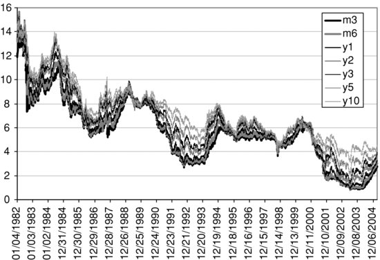
It is evident that rates followed marked trends over the period. From a high of about 15% in 1982, by the end of the same period the short-term rates were below 3%. Also, periods where the term structure of interest rates is relatively flat are interspersed with periods when the term structure is upward sloping, sometimes with the long-term rates being several percent higher than the short-term rates. During the upward sloping yield curve regimes, especially the latter one from 2000 to 2005, the medium- to long-term interest rates are more volatile than the short-term rates, in absolute terms. However, it is not clear which rates are the most volatile in relative terms, as the short rates are much lower than the medium to long-term rates. There are three decisions that must be made:

Decision 1: How Long a Historical Data Period Should Be Used?

The equally weighted historical method gives an average volatility, or correlation, over the sample period chosen. The longer the data period, the less relevant that average may be today (that is, at the end of the sample). Looking at Figure 4, it may be thought that data from 2000 onward, and possibly also data during the first half of the 1990s, are relevant today. However, we may not wish to include data from the latter half of the 1990s, when the yield curve was flat.

Decision 2: Which Frequency of Observations Should Be Used?

This is an important decision, which depends on the end use of the covariance matrix. We can always use the square root of time rule to convert the holding period of a covariance matrix. For instance, a 10-day covariance matrix can be converted into a 1-day matrix by dividing each element by 10; and it can be converted into an annual covariance matrix by multiplying each element by 25. However, this conversion is based on the assumption that variations in interest rates are independent and identically distributed. Moreover, the data become more noisy when we use high-frequency data. For instance, daily variations may not be relevant if we only ever want to measure covariances over a 10-day period. The extra variation in the daily data is not useful, and the crudeness of the square root of time rule will introduce an error. To avoid the use of crude assumptions it is best to use a data frequency that corresponds to the holding period of the covariance matrix.

However, the two decisions above are linked. For instance, if data are quarterly, we need a data period of five or more years; otherwise, the standard error of the estimates will be very large. But then our quarterly covariance matrix represents an average over many years that may not be thought of as relevant today. If data are daily, then just one year of data provides plenty of observations to measure the historical model volatilities and correlations accurately. Also, a history of one year is a better representation of today's markets than a history of five or more years. However, if it is a quarterly covariance matrix that we seek, we have to apply the square root of time rule to the daily matrix. Moreover, the daily variations that are captured by the matrix may not be relevant information at the quarterly frequency.

In summary, there may be a trade-off between using data at the relevant frequency and using data that are relevant today. It should be noted that such a trade-off between Decisions 1 and 2 above applies to the measurement of risk in all asset classes and not only to interest rates.

In interest rates, there is another decision to make before we can measure risk. Since the price value of a basis point (PV01) sensitivity vector is usually measured in basis points, an interest rate covariance matrix is also usually expressed in basis points. Hence, we have Decision 3.

Decision 3: Absolute versus Relative Measures

Should the volatilities and correlations be measured directly on absolute changes in interest rates, or should they be measured on relative changes and then the result converted into absolute terms?

If rates have been trending over the data period the two approaches are likely to give very different results. One has to make a decision about whether relative changes or absolute changes are the more stable. In these data, for example, an absolute change of 50 basis points in 1982 was relatively small, but in 2005 it would have represented a very large change. Hence, to estimate an average daily covariance matrix over the entire data sample, it may be more reasonable to suppose that the volatilities and correlations should be measured on relative changes and then converted to absolute terms.

Note, however, that a daily matrix based on the entire sample would capture a very long-term average of volatilities and correlations between daily U.S. Treasury rates, indeed it is a 22-year average that includes several periods of different regimes in interest rates. Such a long-term average, which is useful for long-term forecasts, may be better based on lower frequency data (e.g., monthly). For a 1-day forecast horizon, we shall use only the data since January 1, 2000.

To make the choice for Decision 3, we take both the relative daily changes (the difference in the log rates) and the absolute daily changes (the differences in the rates, in basis-point terms). Then we obtain the standard deviation, correlation, and covariance in each case, and in the case of relative changes we translate the results into absolute terms. We now compare results based on relative changes with results based on absolute changes. The correlation matrix estimates based on the period January 1, 2000, to March 11, 2005, are shown in Table 1.

Table 1 Correlation of U.S. Treasuries

The matrices are similar. Both matrices display the usual characteristics of an interest rate term structure: Correlations are higher at the long end than the short end, and they decrease as the difference between the two maturities increases.

Table 2 compares the volatilities of the interest rates obtained using the two methods. The figures in the last row of each table represent an average absolute volatility for each rate over the period January 1, 2000 to March 11, 2005. Basing this first on relative changes in interest rates, Table 2(a) gives the standard deviation of relative returns volatility in the first row. The long-term rates have the lowest standard deviations, and the medium-term rates have the highest standard deviations. These standard deviations are then annualized (by multiplying by √250, assuming each rate is independent and identically distributed) and multiplied by the level of the interest rate on March 11, 2005. There was a very marked upward sloping yield curve on March 11, 2005. Hence the long-term rates are more volatile than the short-term rates: For instance, the 3-month rate has an absolute volatility of about 76 basis points, but the absolute volatility of the 10-year rates is about 98 basis points.

Table 2 Volatility of U.S. Treasuries

Table 2(b) measures the standard deviation of absolute changes in interest rates over the period January 1, 2000 to March 11, 2005, and then converts this into volatility by multiplying by √ 250. We again find that the long-term rates are more volatile than the short-term rates; for instance, the six-month rate has an absolute volatility of about 62 basis points, but the absolute volatility of the five-year rates is about 106 bps. (It should be noted that it is quite unusual for long-term rates to be more volatile than short-term rates. But from 2000 to 2004 the U.S. Fed was exerting a lot of control on short-term rates, to bring down the general level of interest rates. However, the market expected interest rates to rise, because the yield curve was upward sloping during most of the period.) We find that correlations were similar, whether based on relative or absolute changes. But Table 2 shows there is a substantial difference between the volatilities obtained using the two methods. When volatilities are based directly on the absolute changes, they are slightly lower at the short end and substantially lower for the medium-term rates.

Table 3 One-Day Covariance Matrix of U.S. Treasuries, in Basis Points

Finally, we obtain the annual covariance matrix of absolute changes (in basis point terms) by multiplying the correlation matrix by the appropriate absolute volatilities and to obtain the one-day covariance matrix we divide by 250. The results are shown in Table 3. Depending on whether we base estimates of volatility and correlation on relative or absolute changes in interest rates, the covariance matrix can be very different. In this case, it is short-term and medium-term volatility estimates that are the most affected by the choice. Given that we have used the equally weighted average methodology to construct the covariance matrix, the underlying assumption is that volatilities and correlations are constant. Hence, the choice between relative or absolute changes depends on which are the more stable. In countries with very high interest rates, or when interest rates have been trending during the sample period, relative changes tend to be more stable than absolute changes.

In summary, there are four crucial decisions to be made when estimating a covariance matrix for interest rates:

The first three decisions must also be made when estimating covariance matrices in other asset classes such as equities, commodities, and foreign exchange rates. There is a huge amount of model risk involved with the construction of covariance matrices; very different results may be obtained depending on the choice made.

Pitfalls of the Equally Weighted Moving Average Method

The problems encountered when applying this model stem not from the small jumps that are often encountered in financial asset prices, but from the large jumps that are only rarely encountered. When a long averaging period is used, the importance of a single extreme event is averaged out within a large sample of returns. Hence, a moving average volatility estimate may not respond enough to a short, sharp shock in the market. This effect is clearly visible in 2002, where only the 30-day volatility rose significantly over a matter of a few weeks. The longer-term volatilities did rise, but it took several months for them to respond to the market falls in the MIB during mid-2002. At this point in time there was actually a cluster of volatility, which often happens in financial markets. The effect of the cluster was to make the longer-term volatilities rise, eventually, but then they took too long to return to normal levels. It was not until markets returned to normal in late 2003 that the three volatility series in Figure 2 are in line with each other.

When there is an extreme event in the market, even just one very large return will influence the T-day moving average estimate for exactly T days until that very large squared return falls out of the data window. Hence volatility will jump up, for exactly T days, and then fall dramatically on day T + 1, even though nothing happened in the market on that day. This type of ghost feature is simply an artifact of the use of equal weighting. The problem is that extreme events are just as important to current estimates, whether they occurred yesterday or a very long time ago. A single large, squared return remains just as important T – 1 days ago as it was yesterday. It will affect the T-day volatility or correlation estimate for exactly T days after that return was experienced, and to exactly the same extent. However, with other models we would find that volatility or correlation had long ago returned to normal levels. Exactly T + 1 days after the extreme event, the equally weighted moving average volatility estimate mysteriously drops back down to about the correct level—that is, provided that we have not had another extreme return in the interim!

Note that the smaller is T, the number of data points used in the data window, the more variable the historical volatility series will be. When any estimates are based on a small sample size they will not be very precise. The larger the sample size the more accurate the estimate, because sampling errors are proportional to 1/√T. For this reason alone a short moving average will be more variable than a long moving average. Hence, a 30-day historic volatility (or correlation) will always be more variable than a 60-day historic volatility (or correlation) that is based on the same daily return data. Of course, if one really believes in the assumption of constant volatility that underlies this method, one should always use as long a history as possible, so that sampling errors are reduced.

It is important to realize that whatever the length of the historical averaging period and whenever the estimate is made, the equally weighted method is always estimating the same parameter: the unconditional volatility (or correlation) of the returns. But this is a constant—it does not change over the process. Thus, the variation in T-day historic estimates can only be attributed to sampling error: There is nothing else in the model to explain this variation. It is not a time-varying volatility model, even though some users try to force it into that framework.

The problem with the equally weighted moving average model is that it tries to make an estimate of a constant volatility into a forecast of a time-varying volatility. Similarly, it tries to make an estimate of a constant correlation into a forecast of a time-varying correlation. No wonder financial firms have lost a lot of money with this model! It is really only suitable for long-term forecasts of average volatility, or correlation, for instance over a period of between six months to several years. In this case, the look-back period should be long enough to include a variety of price jumps, with a relative frequency that represents the modeler expectations of the probability of future price jumps of that magnitude during the forecast horizon.

Using Equally Weighted Moving Averages

To forecast a long-term average for volatility using the equally weighted model, it is standard to use a large sample size T in the variance estimate. The confidence intervals for historical volatility estimators given earlier in this entry provide a useful indication of the accuracy of these long-term volatility forecasts and the approximate standard errors that we have derived earlier in this entry give an indication of variability in long-term volatility. Here, we saw that the variability in estimates decreased as the sample size increased. Hence, long-term volatility that is forecast from this model may prove useful.

When pricing options, it is the long-term volatility that is most difficult to forecast. Options trading often focuses on short-maturity options and long-term options are much less liquid. Hence, it is not easy to forecast a long-term implied volatility. Long-term volatility holds the greatest uncertainty, yet it is the most important determinant of long-term option prices.

We conclude this section with an interesting conundrum, considering two hypothetical historical volatility modelers, whom we shall call Tom and Dick, both forecasting volatility over a 12-month risk horizon based on equally weighted average of squared returns over the past 12 months of daily data. Imagine that it is January 2006 and that on October 15, 2005, the market crashed, returning –50% in the space of a few days. So some very large jumps occurred during the current data window, albeit three months ago.

Tom includes these extremely large returns in his data window, so his ex-post average of squared returns, which is also his volatility forecast in this model, will be very high. Because of this, Tom has an implicit belief that another jump of equal magnitude will occur during the forecast horizon. This implicit belief will continue until one year after the crash, when those large negative returns fall out of his moving data window. Consider Tom's position in October 2006. Up to the middle of October he includes the crash period in his forecast but after that the crash period drops out of the data window and his forecast of volatility in the future suddenly decreases—as if he suddenly decided that another crash was very unlikely. That is, he drastically changes his belief about the possibility of an extreme return. So, to be consistent with his previous beliefs, should Tom now “bootstrap” the extreme returns experienced during October 2005 back into his data set?

And what about Dick, who in January 2006 does not believe that another market crash could occur in his 12-month forecast horizon? So, in January 2006, he should somehow filter out those extreme returns from his data. Of course, it is dangerous to embrace the possibility of bootstrapping in and filtering out extreme returns in data in an ad hoc way, before it is used in the model. However, if one does not do this, the historical model can imply a very strange behavior of the beliefs of the modeler.

In the Bayesian framework of uncertain volatility the equally weighted model has an important role to play. Equally weighted moving averages can be used to set the bounds for long-term volatility; that is, we can use the model to find a range [σmin, σmax] for the long-term average volatility forecast. The lower bound σmin can be estimated using a long period of historical data with all the very extreme returns removed and the upper bound σmax can be estimated using the historical data where the very extreme returns are retained—and even adding some!

A modeler's beliefs about long-term volatility can be formalized by a probability distribution over the range [σmin, σmax]. This distribution would then be carried through for the rest of the analysis. For instance, upper and lower price bounds might be obtained for long-term exposures with option-like structures, such as warrants on a firm's equity or convertibles bonds. This type of Bayesian method, which provides a price distribution rather than a single price, will be increasingly used in market risk management in the future.

EXPONENTIALLY WEIGHTED MOVING AVERAGES

An exponentially weighted moving average (EWMA) avoids the pitfalls explained in the previous section because it puts more weight on the more recent observations. Thus as extreme returns move further into the past as the data window slides along, they become less important in the average.

Statistical Methodology

An exponentially weighted moving average can be defined on any time series of data. Say that on date t we have recorded data up to time t − 1, so we have observations (xt – 1, … . , x1). The exponentially weighted average of these observations is defined as:

where λ is a constant, 0 < λ < 1, called the smoothing or the decay constant. Since λT → 0 as T → ∞ the exponentially weighted average places negligible weight on observations far in the past. And since 1 + λ + λ2 +.... = (1 − λ)−1 we have, for large t,

This is the formula that is used to calculate exponentially weighted moving average (EWMA) estimates of variance (with x being the squared return) and covariance (with x being the cross product of the two returns). As with equally weighted moving averages, it is standard to use squared daily returns and cross products of daily returns, not in mean deviation form. That is:

(19)

and

(20)

The above formulas may be rewritten in the form of recursions, more easily used in calculations:

(21)

and

(22)

An alternative notation used for the above is when we want to make explicit the dependence on the smoothing constant.

One converts the variance to volatility by taking the annualized square root, the annualizing constant being determined by the data frequency as usual. Note that for the EWMA correlation the covariance is divided by the square root of the product of the two EWMA variance estimates, all with the same value of λ. Similarly for the EWMA beta the covariance between the stock (or portfolio) returns and the market returns is divided by the EWMA estimate for the market variance, both with the same value of λ. That is:

(23)

and

(24)

Figure 5 EWMA Volatility Estimates for SP100 with Different λs

Interpretation of λ

There are two terms on the right-hand side of (21). The first term determines the intensity of reaction of volatility to market events: The smaller is λ the more the volatility reacts to the market information in yesterday's return. The second term determines the persistence in volatility: Irrespective of what happens in the market, if volatility was high yesterday it will be still be high today. The closer that λ is to 1, the more persistent is volatility following a market shock.

Thus, a high λ gives little reaction to actual market events but great persistence in volatility, and a low λ gives highly reactive volatilities that quickly die away. An unfortunate restriction of exponentially weighted moving average models is that the reaction and persistence parameters are not independent: The strength of reaction to market events is determined by 1 – λ, while the persistence of shocks is determined by λ. But this assumption is not empirically justified except perhaps in a few markets (e.g., major U.S. dollar exchange rates).

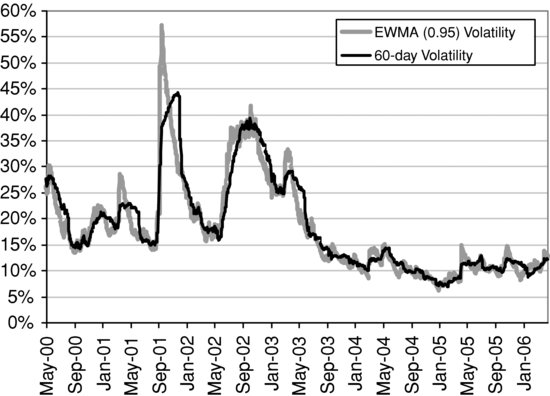
Figure 6 EWMA versus Equally Weighted Volatility

The effect of using a different value of λ in EWMA volatility forecasts can be quite substantial. Figure 5 compares two EWMA volatility estimates/forecasts of the S&P 100 index, with λ = 0.90 and λ = 0.975. It is not unusual for these two EWMA estimates to differ by as much as 10%.

So which is the best value to use for the smoothing constant? How should we choose λ? This is not an easy question. (By contrast, in generalized autoregressive conditional heteroskedascity (GARCH) models there is no question of how we should estimate parameters, because maximum likelihood estimation is an optimal method that always gives consistent estimators.) Statistical methods may be considered: For example, λ could be chosen to minimize the root mean square error between the EWMA estimate of variance and the squared return. But, in practice, λ is often chosen subjectively because the same value of λ has to be used for all elements in an EWMA covariance matrix. As a rule of thumb, we might take values of λ between about 0.75 (volatility is highly reactive but has little persistence) and 0.98 (volatility is very persistent but not highly reactive).

Properties of the Estimates

An EWMA volatility estimate will react immediately following an unusually large return, then the effect of this return on the EWMA volatility estimate gradually diminishes over time. The reaction of EWMA volatility estimates to market events therefore persists over time, and with a strength that is determined by the smoothing constant λ. The larger the value of λ, the more weight is placed on observations in the past and so the smoother the series becomes.

Figure 6 compares the EWMA volatility of the MIB index with λ = 0.95 and the 60-day equally weighted volatility estimate. The difference between the two estimators is marked following an extreme market return. The EWMA estimate gives a higher volatility than the equally weighted estimate, but it returns to normal levels faster than the equally weighted estimate because it does not suffer from the ghost features discussed above.

One of the disadvantages of using EWMA to estimate and forecast covariance matrices is that the same value of λ is used for all the variances and covariances in the matrix. For instance, in a large matrix covering several asset classes, the same λ applies to all equity indexes, foreign exchange rates, interest rates, and/or commodities in the matrix. But why should all these risk factors have similar reaction and persistence to shocks? This constraint is commonly applied merely because it guarantees that the matrix will be positive semidefinite.

The EWMA Forecasting Model

The exponentially weighted average variance estimate (19), or in its equivalent form (21), is just a methodology for calculating . That is, it gives a variance estimate at any point in time but there is no model as such that explains the behavior of the variance of returns, at each time t. In this sense, we have to distinguish EWMA from a GARCH model, which starts with a proper specification of the dynamics of and then proceeds to estimate the parameters of this model.

Without a proper model, it is not clear how we should turn our current estimate of variance into a forecast of variance over some future horizon. One possibility is to augment (21) by assuming it is the estimate associated with the model

(25)

An alternative is to assume a constant volatility, so the fact that our estimates are time varying is merely due to sampling error. In that case any EWMA variance forecast must be constant and equal to the current EWMA estimate. Similar remarks apply to the EWMA covariance, this time regarding EWMA as a simplistic version of bivariate normal GARCH. Similarly, the EWMA volatility (or correlation) forecast for all risk horizons is simply set at the current EWMA estimate of volatility (or correlation). The base horizon for the forecast is given by the frequency of the data—daily returns will give the one-day covariance matrix forecast, weekly returns will give the one-week covariance matrix forecast, and so forth. Then, since the returns are independent and identically distributed, the square root of time rule applies. So we can convert a one-day forecast into an h-day covariance matrix forecast by multiplying each element of the one-day EWMA covariance matrix by h.

Since the choice of λ itself is quite ad hoc, as discussed above, some users choose different values of λ for forecasting over different horizons. For instance, as discussed later in this entry, in the RiskMetricsTM methodolgy a relatively low value of λ is used for short-term forecasts and a higher value of λ is used for long-term forecasts. However, this is purely an ad hoc rule.

Standard Errors for EWMA Forecasts

In the previous section, we justified the assumption that the underlying returns are normally and independently distributed with mean zero and variance σ2. That is, for all t

In this section, we use this assumption to obtain standard errors for EWMA forecasts. From the above, and further from the normality assumption, we have:

Now we can apply the variance operator to (21) and calculate the variance of the EWMA variance estimator as:

(26)

For instance, as a percentage of the variance, the standard error of the EWMA variance estimator is about 5% when λ = 0.95, 10.5% when λ = 0.9, and 16.2% when λ = 0.85.

A single point forecast of volatility can be very misleading. A forecast is always a distribution. It represents our uncertainty over the quantity that is being forecast. The standard error of a volatility forecast is useful because it can be translated into a standard error for a VaR estimate, for instance, or an option price. In any VaR model one should be aware of the uncertainty that is introduced by possible errors in the forecast of the covariance matrix. Similarly, in any mark-to-model value of an option, one should be aware of the uncertainty that is introduced by possible errors in the volatility forecast.

The RiskMetrics™ Methodology

Three very large covariance matrices, each based on a different moving average methodology, are available from www.riskmetrics.com. These matrices cover all types of assets including government bonds, money markets, swaps, foreign exchange, and equity indexes for 31 currencies and commodities. Subscribers have access to all of these matrices updated on a daily basis—and end-of-year matrices are also available to subscribers wishing to use them in scenario analysis. After a few days, the datasets are also made available free for educational use.

The RiskMetrics™ group is the market leader in market and credit risk data and modeling for banks, corporate asset managers, and financial intermediaries. It is highly recommended that readers visit the Web site (www.riskmetrics.com), where they will find a surprisingly large amount of information in the form of free publications and data. See the References at the end of this entry for details.

The three covariance matrices provided by the RiskMetrics group are each based on a history of daily returns in all the asset classes mentioned above. They are:

The main difference between the three different methods is evidenced following major market movements: The regulatory forecast will produce a ghost effect of this event, and does not react as much as the daily or monthly forecasts. The most reactive is the daily forecast, but it also has less persistence than the monthly forecast.

Figure 7 compares the estimates for the FTSE 100 volatility based on each of the three RiskMetrics methodologies and using daily data from January 2, 1995, to June 23, 2006. As mentioned earlier in this entry, these estimates are assumed to be the forecasts over, respectively, one day, one month, and one year. In volatile times, the daily and monthly estimates lie well above the regulatory forecast and the converse is true in more tranquil periods. For instance, during most of 2003, the regulatory estimate of average volatility over the next year was about 10% higher than both of the shorter-term estimates. However, it was falling dramatically during this period, and indeed the regulatory forecast of more than 20% volatility on average between June 2003 and June 2004 was entirely wrong. However, at the end of the period, in June 2006, the daily forecasts were above 20%, and the monthly forecasts were only just below this. However, the regulatory forecast over the next year was only slightly more than 10%.

Figure 7 Comparison of the RiskMetrics “Forecasts” for FTSE100 Volatility

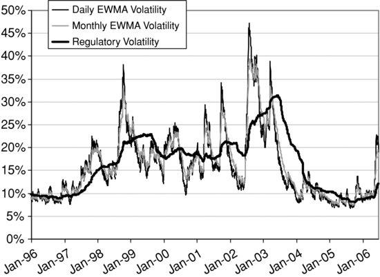
During periods when the markets have been tranquil for some time, for instance during the whole of 2005, the three forecasts tend to agree more. But during and directly after a volatile period there are large differences between the regulatory forecasts and the two EWMA forecasts, and these differences are very difficult to justify. Neither the equally weighted average nor the EWMA methodology is based on a proper forecasting model. One simply assumes the current estimate is the volatility forecast. But the current estimate is a backward-looking measure based on recent historical data. So both of these moving average models make the assumption that the behavior of future volatility is the same as its past behavior and this is a very simplistic view.

KEY POINTS

• The equally weighted moving average, or historical approach to estimating/forecasting volatilities and correlations, was the only statistical method used by practitioners until the mid-1990s.
• The historical method may provide a useful indication of the possible range for a long-term average, such as the average volatility or correlation over the next several years. However, its application to short-term forecasting suffers from at least four drawbacks: (1) The forecast of volatility/correlation over all future horizons is simply taken to be the current estimate of volatility, because the underlying assumption in the model is that returns are independent and identically distributed; (2) the only choice facing the user is on the data points to use in the data window; (3) following an extreme market move the forecasts of volatility and correlation will exhibit a so-called “ghost” feature of that extreme move, which will severely bias the volatility and correlation forecasts upward; and (4) the extent of this bias depends very much on the size of the data window.
• The bias issue associated with the historical approach was addressed by the RiskMetrics™ data and software suite. The choice of methodology helped to popularize the use of exponentially weighted moving averages (EWMA) by financial analysts.
• The EWMA approach provides useful forecasts for volatility and correlation over the very short term, such as over the new day or week. However, its use for longer-term forecasting is limited, and this methodology has two major problems: (1) The forecast of volatility/correlation over all future horizons is simply taken to be the current estimate of volatility, because the underlying assumption in the model is that returns are independent and identically distributed, and (2) the only choice facing the user is about the value of the smoothing constant. With the EWMA approach, the forecasts produced depend crucially on this decision, yet there is no statistical procedure to choose for the value of the smoothing constant.
• Moving average models assume returns are independent and identically distributed, and the further assumption that they are normally distributed allows one to derive standard errors and confidence intervals for moving average forecasts. But empirical observations suggest that returns to financial assets are hardly ever independent and identically, let alone normally, distributed. For these reasons more and more practitioners are basing their forecasts on generalized autoregressive conditional heteroskedasticity (GARCH) models.
• There is no doubt that GARCH models produce superior volatility forecasts. It is only in GARCH models that the term structure volatility forecasts converge to the long-run average volatility—the other models produce constant volatility term structures. Moreover, the value of the EWMA smoothing constant is chosen subjectively and the same smoothing constant must be used for all the returns, otherwise the covariance matrix need not be positive semidefinite. But GARCH parameters are estimated optimally and GARCH covariance matrices truly reflect the time-varying volatilities and correlations of the multivariate returns distributions.

REFERENCES

Alexander, C. (2008a). Market Risk Analysis. Volume I: Quantitative Methods in Finance. Chichester, UK: John Wiley & Sons.

Alexander, C. (2008b). Market Risk Analysis. Volume II: Practical Financial Econometrics. Chichester, UK: John Wiley & Sons.

Freund, J. E. (1998). Mathematical Statistics. Englewood Cliffs: Pearson U.S. Imports & PHIPEs.

RiskMetrics (1996). RiskMetrics Technical Document, http://www.riskmetrics.com/rmcovv.html.

RiskMetrics (1999). Risk Management—A Practical Guide, http://www.riskmetrics.com/pracovv.html.

RiskMetrics (2001). Return to RiskMetrics: The Evolution of a Standard, http://www.riskmetrics.com/r2rovv.html.