
Estimate of Downside Risk with Fat-Tailed and Skewed Models
The financial crisis of 2008 has led many practitioners and academics to reassess the adequacy of the return distribution models, in particular, the left tail. This entry focuses on modeling the left fat tails since they reflect market crashes or crises and play an essential role in downside risk management.
The most common model of asset returns is assumed to be normally or Gaussian distributed (see Bachelier, 1900). In other words, the returns follow a random walk or Brownian motion. This model is natural if one assumes the return over a time interval to be the result of many small independent shocks, which leads to a Gaussian distribution by the central limit theorem. However, empirical studies have observed that the return distributions are more leptokurtic or fat-tailed than Gaussian distributions.
A normal distribution model assumes that an asset return that is three standard deviations below its arithmetic mean (popularly referred to as a “three-sigma event”) has a probability of only approximately 0.13%; that is, once every 1,000 times. For example, from January 1926 to March 2010, the S&P 500 total return index had a monthly mean return of 0.93% and a monthly standard deviation of 5.54%. A negative three-sigma event would be a return lower than −15.69%. During this time period of 1,010 months, there were 10 monthly returns worse than −15.69% as shown in Table 1 (the three-sigma event), with the most recent loss of −16.79% in October 2008 being ranked at ninth. This implies the probability of a three-sigma event is about 1% rather than 0.13%, or eight times greater than we would expect under a normal distribution. Hence, a normal distribution fails to describe the “fat” or “heavy” tails of the stock market.
Table 1 The Worst 10 Monthly Returns for the S&P 500 (from 1/1926 to 3/2010)
| S&P 500 (%) | |
| Sep 1931 | −29.73 |
| Mar 1938 | −24.87 |
| May 1940 | −22.89 |
| May 1932 | −21.96 |
| Oct 1987 | −21.52 |
| Apr 1932 | −19.97 |
| Oct 1929 | −19.73 |
| Feb 1933 | −17.72 |
| Oct 2008 | −16.79 |
| Jun 1930 | −16.25 |
| Source: Morningstar Encorr. | |
Many statistical models have been put forth to account for the heavy tails. We discuss several standard and popular fat-tailed models, such as Mandelbrot's Lévy stable hypothesis (see Mandelbrot, 1963), the Student's t-distribution (see Blattberg and Gonedes, 1974), the mixture of normal distributions (see Clark, 1973), and GARCH (see Bollerslev, 1986) models. There are many other fat-tailed candidates, and this entry does not aim at being exhaustive. Instead, we select representative models and illustrate them through examples so that practitioners may have some intuition about these practically implementable models.
Along the way, we introduce a relatively new fat-tailed and skewed model: the truncated Lévy flight (TLF). Another name for the TLF is the tempered stable distribution. The TLF model has a few interesting properties that we will illustrate later, such as possessing fat tails, skewness, finite moments, and time scaling. Of course, these quantitative models are not the only tool, and they need to be integrated with judgmental analyses and other estimates, but they represent a good starting point for the management of downside risk.
DOWNSIDE RISK MEASURE
Before we dive into the discussions of fat-tailed models, we need to specify an appropriate downside risk measure. A popular downside risk measure is value-at-risk (VaR), which is an estimate of the loss that we expect to be exceeded with a given level of probability (e.g., 5%) over a specified time period. VaR has been recommended as a way of measuring risk by regulators and various financial industry advisory committees.
Conditional value-at-risk (CVaR), a closely related measure to VaR, is derived by taking a weighted average between the VaR and losses exceeding the VaR. Other terms for CVaR include mean shortfall, tail VaR, and expected tail loss. Studies such as Rockafellar and Uryasev (2000), for example, have shown that CVaR has more attractive properties than VaR. Specifically, CVaR is a coherent measure of risk as proved by Pflug (2000) in the sense of Artzner et al. (1999). One of the coherent measures is subadditivity; that is, the risk of a combination of investments is at most as large as the sum of the individual risks. VaR is not always subadditive, which means that the VaR of a portfolio with two instruments may be greater than the sum of individual VaRs of these two instruments. In contrast, CVaR is subadditive. Therefore, CVaR is a more appropriate measure of downside risk.
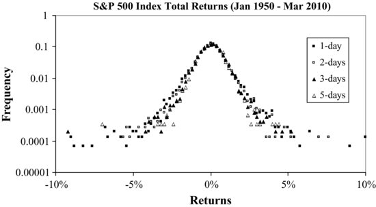
Figure 1 The Time Scaling of the S&P 500 Index with a Stability Index α = 1.5
LÉVY STABLE DISTRIBUTION
Lévy distributions are stable; that is, the sum of two independent random variables, characterized by the same Lévy distribution of tail index α, is itself characterized by a Lévy distribution of the same index. In other words, the functional form of the distribution is maintained, if we sum up independent, identically distributed Lévy stable random variables. The characteristic function of the Lévy stable distribution is (Lévy, 1925):
The probability density function is obtained by performing the inverse Fourier transform on the characteristic function. The four parameters associated with the Lévy stable distribution are: α determines the tail weight or the distribution's kurtosis with 0 < α ≤ 2; β determines the distribution's skewness; γ is a scale parameter; and δ is a location parameter. One can generate univariate stable distributed returns through a numerical software package, for example, written by John Nolan (2009).1 (In his software, the function “stablernd()” takes four parameters, α, β, γ, and δ, and generates random returns that follow a Lévy stable distribution. For empirical analyses, these four parameters can be estimated by the software's function “stablefit()”.)
In 1963, Mandelbrot modeled cotton prices with a Lévy stable process (Mandelbrot, 1963). Mandelbrot observed that in addition to being fat-tailed, the returns show another interesting property: time scaling. This means that the distributions of returns have similar functional forms for different time intervals, ranging from one day to one month. The time scaling property is very appealing as it allows the sum of two independent Lévy stable distributed variables to be stable distributed, with the same stability index α. The normal distribution is a special case of the Lévy stable distribution, and it is scaled in the same way that the sum of two normally distributed variables is also normally distributed.
Figure 1 shows the time scaling of the S&P 500 index returns at time intervals of 1, 2, 3, and 5 days. The scaling variable for a Lévy stable process of index α is ![]() The best fit gives α = 1.5, and a good data collapse can be observed in Figure 1.
The best fit gives α = 1.5, and a good data collapse can be observed in Figure 1.
Mandelbrot's finding was later supported by Fama's study on stocks (Fama, 1965). A Lévy stable distribution model has fat tails and obeys scaling properties, but it has an infinite variance, which conflicts with empirical observations that the return variance is finite. For example, extensive analyses on high-frequency data (ranging from 1 minute to 1 day) for the 1,000 largest companies provided evidence that the returns have finite variance (Gopikrishnan et al., 1998). Infinite variance complicates the task of risk estimation, as well as the application of mean-variance portfolio construction.
Figure 2 The Distributions of S&P 500 Monthly Returns Fitted by the Log-Stable and Lognormal Models
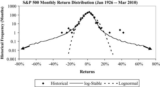
Figure 2 illustrates the log-stable and lognormal distributions in fitting the distribution of monthly S&P 500 returns (also see Martin, Rachev, and Siboulet, 2003). Log-stable distribution applies the stable distribution to log-returns. The vertical axis of Figure 2 is in log scale with a base of 10, and this helps to view the tails of the distribution more clearly. It is clear that the lognormal distribution fails to fit the return distribution below −15% (the above-mentioned three-sigma events). The log-stable distribution fits the tail well, but it extends far beyond the historical maximum loss or gain with nonnegligible probabilities, which eventually results in an infinite variance. In other words, the tail for the log-stable distribution is perhaps too fat.
The infinite variance associated with the stable distribution induces a challenging problem in risk estimation. In practice, what is needed is a model with a distribution falling between the normal and stable distributions so that its tail is appropriately fat, but finite. By truncating the extreme tails of the stable distribution, a model named the truncated Lévy flight has such properties.
Truncated Lévy Flight
The TLF model was first introduced by Mantegna and Stanley (1994) in the physics literature, and it has drawn widespread attention since then. Koponen (1995) modified it in such a way as to allow an analytical calculation of the characteristic function and determination of the complete probability density distribution. Another name for the TLF is the tempered stable distribution—introduced and extended by Boyarchenko and Levendorskii (2000), Carr et al. (2002), Rosinski (2007), and Kim et al. (2008, 2010). Another application is the so-called smoothly truncated stable distribution introduced by Menn and Rachev (2009).
In this entry, we focus on the simplest TLF model by Mantegna and Stanley (1994). The probability density function (PDF) of a simple TLF process is defined as:
where PLevy(x) is the PDF of return x for a Lévy stable distribution and l is the cutoff length for the truncation. It can be seen that the truncation is abrupt. Alternative TLF models are similar and have in general smoother truncations in the form of exponential tails.
Table 2 Parameter Estimates with the Log-TLF Model for Monthly S&P 500, Weekly MSCI EM, and Weekly MSCI EAFE Returns

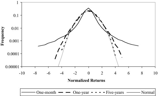
Figure 3 Time Scaling of the TLF process
To simulate a TLF process from a Lévy stable process, we apply a truncation method on the Lévy stable distributed returns generated in the previous section so that the return series follows a TLF model. These truncated returns are then used in the distribution analyses and CVaR estimates, as well as the Monte Carlo simulations.
The truncation is simply implemented, for example, by truncating returns that are beyond 8-sigma for the MSCI Emerging Market index weekly returns or 6.8-sigma for S&P 500 monthly returns. The estimates of the five parameters are shown in Table 2. In the table, we choose the cutoff length in such a way that it is slightly larger than the historical maximum loss (in terms of standard deviation) over the entire historical period. The cutoff length shown in the table is normalized. One can think of a normalized cutoff length of 6 as a six-sigma event. The other four parameters are estimated by the maximum likelihood method.
An interesting feature of the TLF model is its time scaling behavior. Mantegna and Stanley (1994, 1999) show that for a small time interval (e.g., a minute), the TLF distribution approximates a Lévy stable distribution with Lévy stable scaling; while for a significantly large but finite time interval (e.g., a year), the TLF distribution slowly converges to a Gaussian distribution. In other words, the TLF undergoes a crossover from a Lévy stable distribution to a Gaussian distribution as the time interval increases. This crossover is consistent with an independent empirical study of the distribution of daily, weekly and monthly returns for which a progressive convergence to a Gaussian process is deemed to be observed (Akgiray and Booth, 1988).
Figure 3 shows the convergence of the TLF from the Lévy stable distribution at a small time interval to the Gaussian distribution at a large time interval. It shows that as the time interval increases from one month to one year and finally to five years, the normalized return distribution converges from the approximate Lévy stable distribution (one-month interval) to the normal distribution (five-year interval).
The truncation is able to mathematically solve the infinite variance problem inherent in the stable distribution. In fact, the truncation leads to the advantage that all four moments are finite. An interesting question is whether there are economic rationales for the truncation, even though the empirical evidence of finite variance is convincing. The truncation implies an upside or downside boundary for the returns. For the left tail, it is easy to see that the return is bounded by −100% due to limited liability for shareholders for unleveraged indexes or portfolios. However, the existence of the boundary for the upside tail is debatable and it may require extensive separate research. Factors that can limit an infinite positive gain for a large market index such as the S&P 500 may include competitive industries, business cycles, government intervention such as antitrust law and increasing interest rates, contrarian strategies that lead to mean reversion of returns, and so on. Fundamental “intrinsic valuation” indicates that the asset prices should be commensurate with the overall economic growth, which is limited by population growth, labor resources, productivity, and so on.
On the drawback side, like the normal or Lévy stable distribution model, the TLF model assumes an independent and identically distributed process and therefore it cannot describe the time-dependent volatility or volatility clustering observed in market data. Volatility clustering means that a period of high volatility tends to be followed by high volatility and a period of low volatility is likely followed by low volatility.
An attempt to address this drawback is to assume TLF innovations instead of Gaussian innovations in GARCH models. A few studies have investigated the option pricing problem with GARCH dynamics and non-Gaussian innovations. For example, Menn and Rachev (2009) considered smoothly truncated stable innovations in order to provide a practical framework to extend option pricing theory to the Lévy stable model. Kim et al. (2010) studied parametric models based on tempered stable innovations, and they showed that the GARCH model with tempered stable innovations explains both asset price behavior and European option prices better than the normal GARCH model.
STUDENT'S t-DISTRIBUTION
The Student's t-distribution is well documented in the literature. Its probability density function is given by:

where υ is the degrees of freedom. The Student's t-distribution coincides with the Cauchy distribution for υ = 1, and approaches Gaussian for υ → ∞. Finite variance only exists for υ > 2.
Blattberg and Gonedes (1974) proposed that the returns are distributed with a Student's t-distribution. Markowitz and Usmen (1996) found that the daily log-return data of the S&P 500 index can be fitted by the Student's t-distribution with about 4.5 degrees of freedom. Hurst and Platen (1997) reached a similar conclusion. Platen and Sidorowicz (2007) investigated the log-returns of a variety of diversified world stock indexes in different currency denominations by applying the maximum likelihood ratio test to the large class of generalized hyperbolic distributions, and showed that the Student's t-distribution with about four degrees of freedom was the best fit among the models they tested.
The Student's t-distribution is symmetric, thus it cannot model skewness. In order to model negative skewness, Hansen (1994) introduced the skewed Student's t-distribution, which is able to model skewness, but it requires one more parameter to be estimated.
The Student's t-distribution has fat tails but does not obey time scaling, which indicates that the sum of two independent Student's t-distributed variables is not a Student's t-variable with the same degrees of freedom. It cannot model volatility clustering.
The kurtosis of the Student's t distribution is given by ![]() and it is only defined for υ > 4. In other words, the kurtosis is infinite when υ is less than or equal to 4, and the skewness tends to be unstable for υ ≤ 4. In order to avoid an infinite kurtosis, we set the minimum υ as 4.1 when the maximum likelihood estimate gives a value of υ less than 4 (shown as MLE-υ in Table 3). Our numerical simulations show that the CVaR estimate is not sensitive to this small change of υ.
and it is only defined for υ > 4. In other words, the kurtosis is infinite when υ is less than or equal to 4, and the skewness tends to be unstable for υ ≤ 4. In order to avoid an infinite kurtosis, we set the minimum υ as 4.1 when the maximum likelihood estimate gives a value of υ less than 4 (shown as MLE-υ in Table 3). Our numerical simulations show that the CVaR estimate is not sensitive to this small change of υ.
Table 3 Parameter Estimates with the Log Student's t and Log Skewed Student's t Distributions for Monthly S&P 500, Weekly MSCI EM, and Weekly MSCI EAFE Returns
| Log Student's t | ||
| υ | MLE-υ | |
| S&P 500 Monthly | 4.1 | 3.6 |
| MSCI EM Weekly | 4.1 | 4.0 |
| MSCI EAFE Weekly | 4.4 | 4.4 |
| Log Skewed t | ||
| υ | λ | |
| S&P 500 Monthly | 4.1 | −0.13 |
| MSCI EM Weekly | 4.1 | −0.25 |
| MSCI EAFE Weekly | 4.4 | −0.09 |
For the symmetric Student's t-distribution, υ is the only parameter that needs to be estimated for normalized returns. For the skewed Student's t-distribution, we need to add a parameter, λ, to capture the skewness (see Hansen, 1994). These estimated parameters are shown in Table 3.
MIXTURE OF NORMAL DISTRIBUTIONS
In the mixture of normal distributions model, the fat tails are obtained through subordination. The model considered for the log-returns is:
![]()
where μ and σ are associated with the normal process of an individual trade. W is a standard Brownian motion. This model becomes the standard geometric Brownian motion when g(t) is constant. g(t) is a subordinator and positive increasing random process that characterizes the market trading activity time.
If g(t) is assumed to be lognormally distributed with mean μs and standard deviation σs, this mixture process is also referred to as the normal-lognormal mixture. The probability density function for the normal-lognormal mixture is given in Clark (1973).
Other kinds of mixtures exist in the literature, such as a normal-gamma mixture, also referred to as a variance gamma process (Madan and Seneta, 1990). In this entry, we only illustrate the normal-lognormal mixture, one of the simplest mixture models. The estimated parameters for the normal-lognormal mixture are shown in Table 4.
Table 4 Parameter Estimates with the Mixture Distribution for Monthly S&P 500, Weekly MSCI EM, and Weekly MSCI EAFE Returns
The mixture of normal distributions utilizes the concept of a subordinated process. Clark (1973) assumes that trading volume is a plausible measure of the evolution of price dynamics. Indeed, a sizeable literature has demonstrated a strong positive contemporaneous correlation between trading volume and return volatility (see, for example, Andersen, 1996). More specifically, the distribution of log-returns occurring from a given level of trading volume is subordinate to the distribution of an individual trade and directed by the distribution of the trading volume. By assuming the normal distribution for the individual trade and finite moments for the distribution of the trading volume, Clark (1973) proves that the mixed distribution has fat tails with all moments finite.
The mixture of normal distributions is intuitively appealing because it is directly linked to market microstructure such as information flow, trading volume, and number of transactions. The subordinated process premise has also evolved into stochastic volatility that now receives vigorous attention in the finance literature (see Andersen, 1996). In general, mixture of normal distributions has fat tails but does not obey time scaling. A generalized mixture of normal distributions, however, can describe volatility clustering.
GARCH Models
General autoregressive conditional heteroscedasticity (GARCH) models, first introduced by Bollerslev (1986), are now widely employed in financial time-series analyses. In particular, they are used to predict short horizon volatilities (ranging from one day to one month).
The return generating process is based on geometric Brownian motion but with the variance being a time-dependent GARCH(1,1) process, which is defined by the relation:
![]()
where α0, α1, and β1 are the control parameters of the GARCH(1,1) stochastic process. rt is a random variable with zero mean and variance ![]() , and is characterized by a conditional probability density function ft(x), which is arbitrary but is often chosen to be Gaussian. In this entry, the innovation
, and is characterized by a conditional probability density function ft(x), which is arbitrary but is often chosen to be Gaussian. In this entry, the innovation ![]() is assumed to be Gaussian. These three control parameters are estimated by the maximum likelihood method and shown in Table 5.
is assumed to be Gaussian. These three control parameters are estimated by the maximum likelihood method and shown in Table 5.
Table 5 Parameter Estimates with the GARCH(1,1) Model for Monthly S&P 500, Weekly MSCI EM, and Weekly MSCI EAFE Returns
GARCH models assume that volatility changes with time and with past information. Because of the time-dependent volatility, the unconditional distribution of returns exhibit fat tails. GARCH models allow for volatility clustering or autocorrelation in the volatility.
The most popular GARCH model is GARCH (1,1). The scaling properties of GARCH(1,1) are not clear from the theory; however, numerical simulations of GARCH(1,1) with Gaussian innovations show that it fails to describe the scaling properties of high-frequency data (see Mantegna and Stanley, 1999).
GARCH(1,1) processes are unconditionally stationary with finite variance if ![]() 0, and have finite kurtosis if
0, and have finite kurtosis if ![]()
![]() .
.
MODELING RETURN DISTRIBUTIONS FOR MAJOR INDEXES
Applications of the Lévy stable, Student's t, and mixture of normal distribution models in modeling market indexes are well documented (see, for example, Mandelbrot [1963], Clark [1973], Blattberg and Gonedes [1974], Markowitz and Usmen [1996], Hurst and Platen [1997], Martin, Rachev and Siboulet [2003], Platen and Sidorowicz [2007], etc.). The literature offered detailed methodology on how the model parameters are estimated. In some cases, they performed comparisons for these models.
Mantegna and Stanley (1999) studied the TLF model and GARCH(1,1) with Gaussian innovations processes. They found that the TLF model well describes the time scaling, while it is not able to properly describe the volatility clustering. The GARCH(1,1) model seems to be complementary to the TLF: It is able to describe the volatility clustering, but it fails to describe the time scaling. As mentioned earlier, however, the GARCH model with TLF innovations might offer a better solution to the TLF model or GARCH with Gaussian innovations.
Table 6 Statistics Summary for Historical Returns, as Well as Simulated Returns for Lognormal, Log-TLF, Log Student's t, Log Skewed Student's t, Normal-Lognormal Mixture, and GARCH(1,1) Models
Many previous studies have focused on high-frequency data such as daily return data. Here, we are interested in weekly or monthly data because investors typically have a relatively long investment horizon and portfolios are often rebalanced monthly. We apply these fat-tailed models to some well-known weekly or monthly returns of equity indexes. Our test assets include the monthly S&P 500 total return index, the weekly MSCI Emerging Market index, and the weekly MSCI EAFE index. One reason to use weekly data is to have more data points in the tails given that the MSCI indexes have relatively short histories. A few other equity and fixed income indexes, such as the MSCI UK, U.S. Long-Term Government Bond, Muni bonds, and some individual stocks were tested with the same methodologies and the results are similar, so they are not reported (e.g., Xiong, 2010).
We apply the maximum likelihood method to calibrate model parameters as previous studies did. The estimated parameters for the TLF, Student's t, normal-lognormal mixture, and GARCH(1,1) are shown in Tables 2, 3, 4, and 5, respectively. Since we are more interested in modeling downside risk, our goal is to fit the model's tail distribution to the empirical tail distribution in terms of CVaR through Monte Carlo simulations.
Figure 4 The Historical Distributions of S&P 500 Monthly Returns Fitted by the Log-TLF, Log Skewed Student's t, Normal-Lognormal Mixture, GARCH(1,1), and Lognormal Models
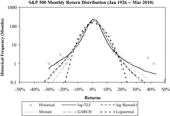
Table 6 focuses on nonstable distribution models and presents the empirical statistics as well as the Monte Carlo simulation results for the six models. The statistics for each model are based on 1,000,000 simulated random returns that follow the corresponding distribution models. It can be seen that the lognormal model underestimates the monthly CVaR by 2.04% for the S&P 500, the weekly CVaR by 1.57% for the MSCI EM, and the weekly CVaR by 0.8% for the MSCI EAFE, respectively. The log Student's t-distribution, normal-lognormal mixture, and GARCH(1,1) have similar CVaR estimates, and all of them are better than the lognormal model but appear to underestimate the tail risk. On the other hand, both the log-TLF model and the log skewed Student's t-model provide a good fit for CVaR for all three indexes: S&P 500, MCSI EM, and MSCI EAFE.
Note that the log Student's t, normal-lognormal mixture, and GARCH(1,1) are positively skewed by design in a way similar to the lognormal distribution because we are working with the log-returns. The positive skewness resulted from taking the exponential function on the log-returns. None of these three models can account for negative skewness without modifications.
Therefore there are two reasons why the log-TLF and the log skewed Student's t-models do well in fitting the CVaR. First, their tails are appropriately fat, and second, both of them are able to capture negative skewness. For the TLF model, the fatness of the tail is controlled by α and the cutoff length and the skewness is controlled by β as shown in Table 2. For the skewed Student's t-distribution, the fatness of the tail is controlled by the degrees of freedom υ and the skewness is controlled by λ as shown in Table 3.
Figures 4, 5, and 6 compare the log-TLF model with other models in fitting the historical return distributions for monthly S&P 500 returns, weekly MSCI EM returns, and weekly MSCI EAFE returns, respectively. The figures confirm the results shown in Table 6. It can be seen that the log-TLF provides a good fit for the three indexes. The log skewed Student's t is almost as effective as the log-TLF model in fitting CVaRs. Compared to the log skewed Student's t-distribution, the log-TLF has a fatter but shorter tail because of the truncation. On the other hand, the normal-lognormal mixture and GARCH(1,1) model have CVaRs that fall between those of the log-TLF and lognormal models. The finding for the log symmetric Student's t-distribution, not plotted due to space limitations, is similar to the normal-lognormal mixture and GARCH(1,1) model.
Figure 5 The Historical Distributions of MSCI EM Weekly Returns Fitted by the Log-TLF, Log Skewed Student's t, Normal-Lognormal Mixture, GARCH(1,1), and Lognormal Models
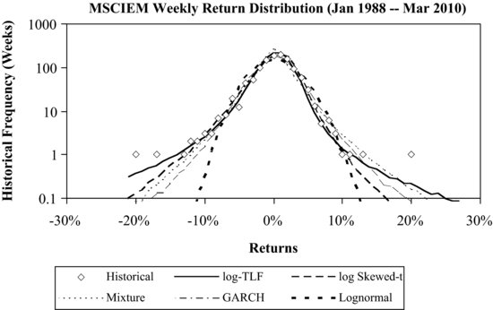
Figure 6 The Historical Distributions of MSCI EAFE Weekly Returns Fitted by the Log-TLF, Log Skewed Student's t, Normal-Lognormal Mixture, GARCH(1,1), and Lognormal Models

Table 7 summarizes the underestimated CVaRs for the six models that have been applied to the three indexes. The underestimated tails are reported on a relative basis based on CVaR estimates shown in Table 6. For example, the lognormal model underestimates the monthly CVaR by a relative percentage of 18% ![]() for the S&P 500 index.
for the S&P 500 index.
Table 7 Underestimated CVaRs in Relative Percentage for the Six Models
Averaging over the three indexes, the lognormal model underestimates the CVaR by about 18% on a relative basis. The normal-lognormal mixture, the log Student's t-distribution, and GARCH(1,1) with Gaussian innovations perform better than the lognormal model but appear to underestimate the CVaR by about 6%, 10%, and 12%, respectively. In contrast, both the log-TLF and log skewed t-distribution did a better job in modeling the CVaR.
KEY POINTS
- It is well known that asset returns often exhibit fat tails, negative skewness, time scaling, and volatility clustering. Fat-tailed and skewed models can be used to estimate the downside risk of assets. It is important that the selected models are able to capture fat tails and skewness, among others.
- The lognormal distribution is the fundamental assumption of many important financial models, but it has thin tails and thus can significantly underestimate the downside risk. On the other side, the Lévy stable distribution exhibits time scaling and fat tails, but it tends to overestimate the downside risk due to its infinite variance.
- The Student's t-distribution can model fat tails but not negative skewness. A modification results in the skewed Student's t-distribution, which can model both fat tails and negative skewness. However, both of them do not possess time scaling properties and cannot model volatility clustering.
- The normal-lognormal mixture is intuitive as it is directly linked to market microstructure such as information flow and trading volume. It has fat tails but cannot model negative skewness. In general, it does not possess time scaling.
- The truncated Lévy flight model can describe the asymptotic return distributions measured at all frequencies and the scaling properties (self-similarities). More specifically, for a small time interval (e.g., a minute), this distribution approximates a Lévy stable distribution with Lévy stable scaling; while for a significantly large but finite time interval (e.g., a year), the truncated Lévy flight distribution slowly converges to a Gaussian distribution. It has finite four moments and can model both fat tails and negative skewness.
- The truncated Lévy flight or tempered stable distribution model cannot describe volatility clustering. In contrast, GARCH with Gaussian innovations can model volatility clustering but it is often found that the tail is not fat enough. Recent studies show that a GARCH with truncated Lévy flight innovations appears to be able to describe most of the stylized empirical facts: fat tails, skewness, and volatility clustering.
NOTE
1. For details, see http://academic2.american.edu/~jpnolan/stable/stable.html/
REFERENCES
Akgiray, V., and Booth, G. G. (1988). The stable-law model of stock returns. Journal of Business & Economic Statistics 6: 51−57.
Anderson, T. (1996). Return volatility and trading volume: An information flow interpretation of stochastic volatility. Journal of Finance 51, 169–204.
Artzner, P., Delbaen, F., Eber, J. M., and Heath, D. (1999). Coherent measures of risk. Mathematical Finance 9, 3: 203–228.
Bachelier, L. (1900). Théorie de la spéculation. Doctoral dissertation. Annales Scientifiques de l’École Normale Supérieure (ii) 17, 21–86. Trans. P. H. Cootner, ed. (1964). The Random Character of Stock Market Prices. Cambridge, MA: MIT Press.
Blattberg, R. C., and Gonedes, N. J. (1974). A comparison of the stable and Student distributions as statistical models for stock prices. Journal of Business 47, 244–280.
Bollerslev, T. (1986). Generalized autoregressive conditional heteroskedasticity. Journal of Econometrics 31, 3: 307–327.
Boyarchenko, S. I., and Levendorskii, S. Z. (2000). Option pricing for truncated Lévy processes. International Journal of Theoretical and Applied Finance 3.
Carr, P., Geman, H., Madan, D., and Yor, M. (2002). The fine structure of asset returns: An empirical investigation. The Journal of Business 75, 2: 305–332.
Clark, P. K. (1973). A subordinated stochastic process model with finite variance for speculative prices. Econometrica 41, 135–155.
Fama, E. F. (1965). The behavior of stock-market prices. The Journal of Business 38, 1: 34–105.
Gopikrishnan, P., Meyer, M., Amaral, L.A.N., and Stanley, H. E. (1998). Inverse cubic law for the distribution of stock price variations. The European Physical Journal B, 3, 2: 139–140.
Hansen, B. E. (1994). Autoregressive conditional density estimation. International Economic Review 35, 705–730.
Hurst, S. R., and Platen, E. (1997). The Marginal Distributions of Returns and Volatility. Lecture Notes—Monograph Series. Vol. 31, L1-Statistical Procedures and Related Topics, pp. 301–314. Institute of Mathematical Statistics.
Kim, Y., Rachev, S., Bianchi, M., and Fabozzi, F. (2008). A new tempered stable distribution and its application to finance. In G. Bol, S. T. Rachev, and R. Würth, (Eds.), Risk Assessment: Decisions in Banking and Finance, pp. 51–84. Physika Verlag, Springer.
Kim, Y., Rachev, S., Bianchi, M., and Fabozzi, F. (2010). Tempered stable and tempered infinitely divisible GARCH models. Journal of Banking and Finance.
Koponen, I. (1995). Analytic approach to the problem of convergence of truncated Lévy flights towards the Gaussian stochastic process. Physical Review E, 52.
Lévy, P. (1925). Calcul des probabilités. Paris: Gauthier-Villars.
Madan, D. B., and Seneta E. (1990). The variance gamma (v.g.) model for share market returns. Journal of Business 63, 511–524.
Mandelbrot, B. (1963). The variation of certain speculative prices. Journal of Business 36, 392–417.
Mantegna, R. N., and Stanley, H. E. (1994). Stochastic process with ultraslow convergence to a Gaussian: The truncated Lévy flight. Physical Review Letters 73, 2946–2949.
Mantegna, R. N., and Stanley, H. E. (1999). An Introduction to Econophysics: Correlations and Complexity in Finance. Cambridge: Cambridge University Press.
Markowitz, H. M., and Usmen, N. (1996). The likelihood of various stock market return distributions, Part 2: Empirical results. Journal of Risk and Uncertainty 13, 3: 221–247.
Martin, R. D., Rachev S., and Siboulet, F. (2003). Phi-alpha optimal portfolios & extreme risk management. Wilmott Magazine of Finance November: 70–83.
Menn, C., and Rachev, S. (2009). Smoothly truncated stable distributions, GARCH-models, and option pricing. Mathematical Methods of Operations Research 63, 3: 411–438.
Nolan, J. (2009). Software Stable 5.1 for MATLAB.
Platen, E., and Sidorowicz, R. (2007). Empirical evidence on Student-t log-returns of diversified world stock indices. Research Paper 194. University of Technology, Sydney. School of Finance and Economics. Quantitative Finance Research Centre.
Pflug, G. Ch. (2000). Some remarks on the value-at-risk and the conditional value-at-risk. In Probabilistic Constrained Optimization: Methodology and Applications, S. Uryasev, (Ed.). New York: Springer.
Rockafellar, R. T., and Uryasev, S. (2000). Optimization of conditional value-at-risk. The Journal of Risk 2, 3: 21–41.
Rosinski, J. (2007). Tempering stable processes. Stochastic Processes and Their Applications 117, 6: 677–707.
Xiong, J. X. (2010). Using truncated Lévy flight to estimate downside risk. Journal of Risk Management in Financial Institutions 3, 3: 231–242.