In Pandas, there is a certain data type for time series data. This is a normal Pandas DataFrame or Series where the index is a column of the datetime objects. It has to be this kind of object for Pandas to recognize it as dates and for it to understand what to do with the dates. To show you how it works, let us read in a time series dataset.

The first data that we are reading in is the mean measured daily temperature at Fisher River near Dallas, USA from 1^st January, 1988 to 31^st December, 1991. The data can be downloaded from DataMarket in several formats ( https://datamarket.com/data/set/235d/ ), and it can also be acquired from http://ftp.uni-bayreuth.de/math/statlib/datasets/hipel-mcleod . Here, I have the data in CSV format. The data comes from the Time Series Data Library ( https://datamarket.com/data/list/?q=provider:tsdl ) and originated in Hipel and McLeod (1994).

The data has two columns: the first with the date and the second with the mean measured temperature on that day. To read in the dates, we need to give a date parsing function to the Pandas CSV data reader, which takes a date in string format and converts it to a datetime object, just as we discussed in previous chapters (for example, Chapter 6, Bayesian Methods). Opening the data file, you can see that the dates are formatted as year-month-day. Thus, we create a date parsing function for this:

dateparse = lambda d: pd.datetime.strptime(d, '%Y-%m-%d')  

With this date parsing function, we can now read in the data as before:

temp = pd.read_csv('data/mean-daily-temperature-fisher-river.csv', 
                   parse_dates=['Date'],  
                   index_col='Date',  
                   date_parser=dateparse) 

As the columns in the file are named, that is, the first row of the data shows Date and Temp, we let the reader know that the index column-the column to take as the index-is the column with the Date name. We also tell it to parse this column with the date parsing function, which is also given by us. Looking at the first few entries, we can see that it is a full DataFrame object:

temp.head() 

To make our analysis easier and as we are working with a univariate dataset, we can extract only the Pandas series out of it. This is just the column in the DataFrame. With the following, we end up with a Series object:

temp = temp.iloc[:,0] 

The Series object still has the dates as index; in fact, printing out the index attribute shows that we have indeed parsed the date as index:

temp.index 

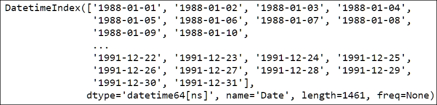
The dtype='datetime64[ns]' value shows that we are storing the index as the date with a very high precision. As always, we first visualize the data to see what we are dealing with:

temp.plot(lw=1.5) 
despine(plt.gca()) 
plt.gcf().autofmt_xdate() 
plt.ylabel('Temperature'), 

As always, these lines simply call the Pandas Series method plot, change the line width (lw), then get the current axis (plt.gca()), which is sent to the despine() function, and then set the y label:

As you can see, there is a strong pattern in the data. As it is repeated in each year, it is a special type of cyclical pattern, a seasonal pattern. To check some of the statistics, we call the describe() method of the Series object that we have:

temp.describe() 

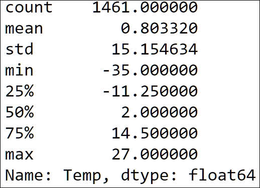
In the printed statistics, we can see that the minimum temperature is -35, pretty cold. We also see that there are a lot of measurements, enough for us to work with, and in time series analysis it is very important to have enough data. When we do not have enough data, we have to employ more sophisticated models such as the judgmental models described in the introduction. We now have time series data to work with, and we will start off with looking at how to slice these objects in Pandas.