
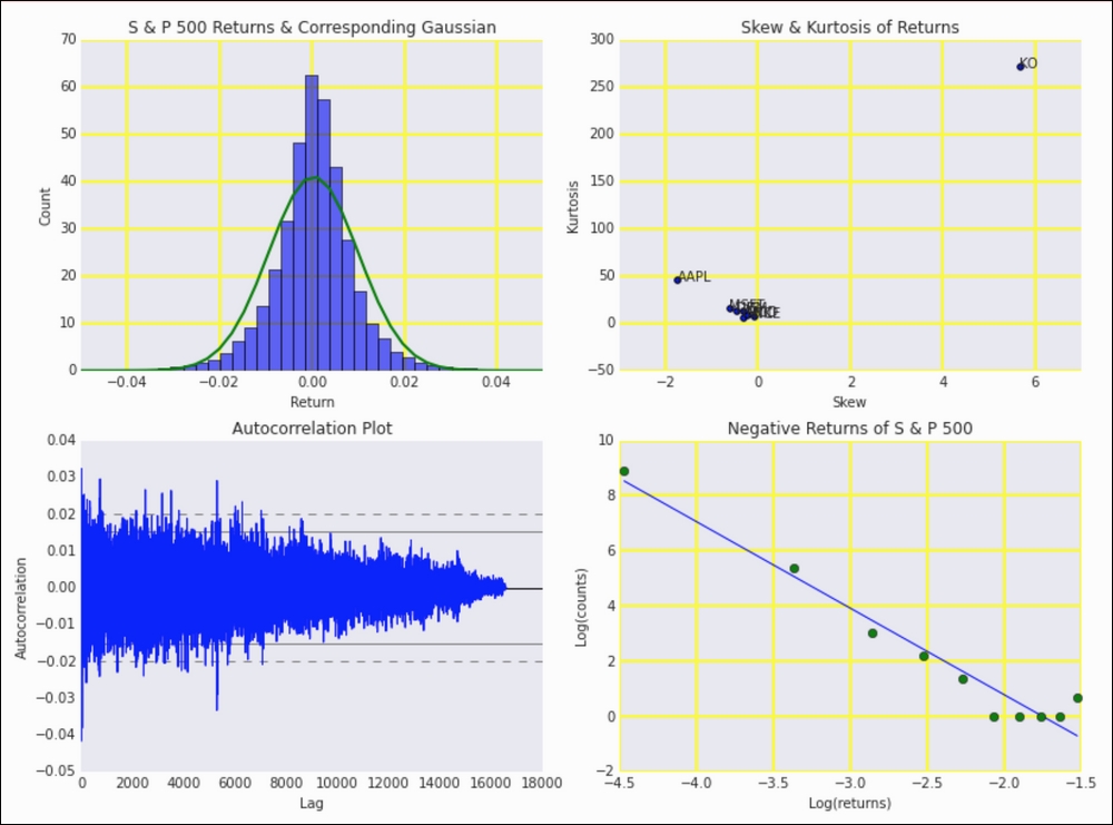
Returns, especially of stock indices, have been extensively studied. In the past, it was assumed that the returns are normally distributed. However, it is now clear that the returns distribution has fat tails (fatter than normal distributions). More information is available at https://en.wikipedia.org/wiki/Fat-tailed_distribution (retrieved October 2015). It is easy enough to check whether data fits the normal distribution. All we need is the mean and standard deviation of the sample.
There are a number of topics that we will explore in this recipe:
- The skewness and kurtosis of stock returns are interesting to study. Skewness is especially important in the context of stock option models. Analysts usually limit themselves to the mean and standard deviation, which are assumed to correspond to reward and risk, respectively.
- If we are interested in the existence of a trend, then we should take a look at an autocorrelation plot. This is a plot of autocorrelation—that is, correlation between a signal and the signal at a certain lag (also explained in Python Data Analysis, Packt Publishing).
- We will also plot negative returns (absolute value thereof) and corresponding counts on a log-log scale, as those approximately seem to follow a power law (especially the tail values).
The analysis can be found in the rets_stats.ipynb file in this book's code bundle:
- The imports are as follows:
import dautil as dl
import ch7util
import matplotlib.pyplot as plt
from scipy.stats import skew
from scipy.stats import kurtosis
from pandas.tools.plotting import autocorrelation_plot
import numpy as np
from scipy.stats import norm
from IPython.display import HTML
- Calculate returns for our stocks:
ohlc = dl.data.OHLC() rets_dict = {} for i, symbol in enumerate(ch7util.STOCKS): rets = ch7util.log_rets(ohlc.get(symbol)['Adj Close']) rets_dict[symbol] = rets sp500 = ch7util.log_rets(ohlc.get('^GSPC')['Adj Close']) - Plot the histogram of the S&P 500 returns and corresponding theoretical normal distribution:
sp = dl.plotting.Subplotter(2, 2, context) sp.ax.set_xlim(-0.05, 0.05) _, bins, _ = sp.ax.hist(sp500, bins=dl.stats.sqrt_bins(sp500), alpha=0.6, normed=True) sp.ax.plot(bins, norm.pdf(bins, sp500.mean(), sp500.std()), lw=2) - Plot the skew and kurtosis of returns:
skews = [skew(rets_dict[s]) for s in ch7util.STOCKS]
kurts = [kurtosis(rets_dict[s]) for s in ch7util.STOCKS]
sp.label()

sp.next_ax().scatter(skews, kurts)
dl.plotting.plot_text(sp.ax, skews, kurts, ch7util.STOCKS)
sp.label()
- Plot the autocorrelation plot of the S&P 500 returns:
autocorrelation_plot(sp500, ax=sp.next_ax())
sp.label()
- Plot the log-log plot of negative returns (absolute value) and counts:
# Negative returns
counts, neg_rets = np.histogram(sp500[sp500 < 0])
neg_rets = neg_rets[:-1] + (neg_rets[1] - neg_rets[0])/2
# Adding 1 to avoid log(0)
dl.plotting.plot_polyfit(sp.next_ax(), np.log(np.abs(neg_rets)),
                         np.log(counts + 1), plot_points=True)
sp.label()

HTML(sp.exit())
Refer to the following screenshot for the end result:
..................Content has been hidden....................
You can't read the all page of ebook, please click here login for view all page.