
When we define a stock market or index, we usually choose stocks that are similar in some way. For instance, the stocks might be in the same country or continent. The position of birds can be roughly estimated from the position of the flock they belong to. Similarly, we expect stock returns to be correlated to their market, although not necessarily perfectly.
We will explore the following metrics:
- The most obvious metric is purportedly the correlation coefficient of the individual stock returns and the S&P 500 index.
- Another metric is the slope obtained from linear regression instead of correlation.
- We can also analyze squared differences of returns somewhat similar to squared errors in regression diagnostics.
- Instead of correlating returns, we can also correlate trading volumes and volatility. To measure volatility, we will use the somewhat uncommon squared value of high and low prices difference. Actually, we are supposed to divide this value by a constant; however, this is not necessary for the correlation coefficient calculation.
The analysis is in the correlating_market.ipynb file in this book's code bundle:
- The imports are as follows:
import ch7util
import dautil as dl
import numpy as np
import matplotlib.pyplot as plt
from IPython.display import HTML
- Define the following function to compute the volatility:
def hl2(df, suffix): high = df['High_' + suffix] low = df['Low_' + suffix] return (high - low) ** 2 - Define the following function to correlate the S&P 500 and our stocks:
def correlate(stock, sp500): merged = ch7util.merge_sp500(stock, sp500) rets = ch7util.log_rets(merged['Adj Close_stock']) sp500_rets = ch7util.log_rets(merged['Adj Close_sp500']) result = {} result['corrcoef'] = np.corrcoef(rets, sp500_rets)[0][1] slope, _ = np.polyfit(sp500_rets, rets, 1) result['slope'] = slope srd = (sp500_rets - rets) ** 2 result['msrd'] = srd.mean() result['std_srd'] = srd.std() result['vols'] = np.corrcoef(merged['Volume_stock'], merged['Volume_sp500'])[0][1] result['hl2'] = np.corrcoef(hl2(merged, 'stock'), hl2(merged, 'sp500'))[0][1] return result - Correlate our set of stocks with the S&P 500 index:
ohlc = dl.data.OHLC() dfs = [ohlc.get(stock) for stock in ch7util.STOCKS] sp500 = ohlc.get('^GSPC') corrs = [correlate(df, sp500) for df in dfs] - Plot correlation coefficients for the stocks:
sp = dl.plotting.Subplotter(2, 2, context) dl.plotting.bar(sp.ax, ch7util.STOCKS, [corr['corrcoef'] for corr in corrs]) sp.label() dl.plotting.bar(sp.next_ax(), ch7util.STOCKS, [corr['slope'] for corr in corrs]) sp.label() - Plot the squared difference statistics:
sp.next_ax().set_xlim([0, 0.001]) dl.plotting.plot_text(sp.ax, [corr['msrd'] for corr in corrs], [corr['std_srd'] for corr in corrs], ch7util.STOCKS, add_scatter=True, fontsize=9, alpha=0.6) sp.label() - Plot volume and volatility correlation coefficients:
dl.plotting.plot_text(sp.next_ax(), [corr['vols'] for corr in corrs],
                      [corr['hl2'] for corr in corrs],
                      ch7util.STOCKS, add_scatter=True,
                      fontsize=9, alpha=0.6)
sp.label()

HTML(sp.exit())
Refer to the following screenshot for the end result:
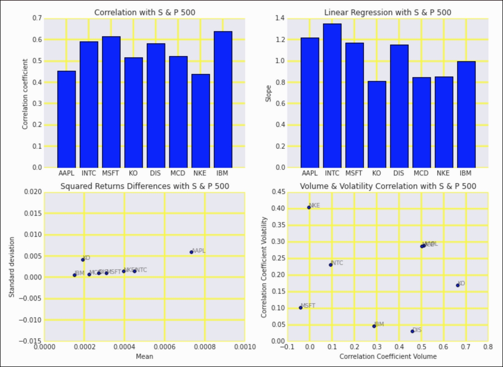
..................Content has been hidden....................
You can't read the all page of ebook, please click here login for view all page.