
In recent 3D games, complex interactions among rigid bodies are ubiquitous. Objects collide with one another, slide on various surfaces, bounce, and roll. The rigid-body dynamic simulation considerably increases the engagement and excitation levels of games. Such examples are shown in Figure 6.3.1. However, without sound induced by these interactions, the synthesized interaction and virtual world are not as realistic, immersive, or convincing as they could be.
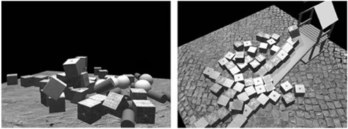
Figure 6.3.1. Complicated interactions among rigid bodies are shown in the two scenes above. In this gem, we introduce how to automatically synthesize sound that closely correlates to these interactions: impact, rolling, and sliding.
Although automatically playing back pre-recorded audio is an effective way for developers to add realistic sound that corresponds well to some specified interactions (for example, collision), it is not practical to pre-record sounds for all the potential complicated interactions that are controlled by players and triggered at run time.
Sound that is synthesized in real time and based on the ongoing physics simulation can provide a much richer variety of audio effects that correspond much more closely to complex interactions.
In this gem, we explore an approach to synthesize contact sounds induced by different types of interactions among rigid bodies in real time. We take advantage of common content resources in games, such as triangle meshes and normal maps, to generate sound that is coherent and consistent with the visual simulation. During the pre-processing stage, for each arbitrary triangle mesh of any sounding object given as an input, we use a modal analysis technique to pre-compute the vibration modes of each object. At run time, we classify contact events reported from physics engines and transform them into an impulse or sequence of impulses, which act as excitation to the modal model we obtained during pre-processing. The impulse generation process takes into consideration visual cues retrieved from normal maps. As a result, sound that closely corresponds to the visual rendering is automatically generated as the audio hardware mixes the impulse responses of the important modes.
In this section, we give a brief overview on the core sound synthesis processes: modal analysis and modal synthesis. Both of them have been covered in previous Game Programming Gems. More details on modal analysis can be found in Game Programming Gems 4 [O’Brien04], and the impulse response to sound calculation (modal synthesis) is described in Game Programming Gems 6 [Singer06].
Figure 6.3.2 shows the pipeline of the sound synthesis module.

Figure 6.3.2. In pre-processing, a triangle mesh is converted into a spring-mass system. Then modal analysis is performed to obtain a bank of vibration modes for the spring-mass system. During run time, impulses are fed to excite the modal bank, and sound is generated as a linear combination of the modes. This is the modal synthesis process.
In the content creation process for games, triangle meshes are often used to represent the 3D objects. In pre-processing, we take these triangle meshes and convert them into spring-mass representations that are used for sound synthesis. We consider each vertex of the triangle mesh as a mass particle and the edge between any two vertices as a damped spring. The physical properties of the sounding objects are expressed in the spring constants of the edges and the masses of the particles. This conversion is shown in Equation (1), where k is the spring constant, Y is the Young’s Modulus that indicates the elasticity of the material, t is the thickness of the object, mi is the mass of particle i, p is the density, and ai is the area covered by particle i.
For more details on the spring-mass system construction, we refer our readers to [Raghuvanshi07].
Since this spring-mass representation is only used in audio rendering and not graphics rendering, the triangle meshes used in this conversion do not necessarily have to be the same as the ones used for graphics rendering. For example, when a large plane can be represented with two triangles for visual rendering, these two triangles do not carry detailed information for approximating the sound of a large plane. (This will be explained later.) In this case, we can subdivide this triangle mesh before the spring-mass conversion and use the detailed mesh for further sound computation. On the contrary, sometimes high-complexity triangle meshes are required to represent some visual details, but we are not necessarily able to hear them. In this scenario, we can simplify the meshes first and then continue with sound synthesis–related computation.
Now that we have a discretized spring-mass representation for an arbitrary triangle mesh, we can perform modal analysis on this representation and pre-compute the vibration modes for this mesh. Vibration of the spring-mass system created from the input mesh can be described with an ordinary differential equation (ODE) system as in Equation (2).
where M, C, and K are the mass, damping, and stiffness matrix, respectively. If there are N vertices in the triangle mesh, r in Equation (1) is a vector of dimension N, and it represents the displacement of each mass particle from its rest position. Each diagonal element in M represents the mass of each particle. In our implementation, C adopts Rayleigh damping approximation, so it is a linear combination of M and K. The element at row i and column j in K represents the spring constant between particle iand particle j. f is the external force vector. The resulting ODE system turns into Equation (3).
where M is diagonal and K is real symmetric. Therefore, Equation (3) can be simplified into a decoupled system after diagonalizing K with K = GDG–1, where D is a diagonal matrix containing the Eigenvalues of K.
The diagonal ODE system that we eventually need to solve is Equation (4).
where Z = G–1r, a linear combination of the original vertex displacement. The general solution to Equation (4) is Equation (5).

where λ is the i’th Eigenvalue of D. With particular initial conditions, we can solve for the coefficient ci and its complex conjugate, ![]() . The absolute value of ωi’s imaginary part is the frequency of that mode. Therefore, the vibration of the original triangle mesh is now approximated with the linear combination of the mode shapes zi. This linear combination is directly played out as the synthesized sound. Since only frequencies between 20 Hz to 20 kHz are audible to human beings, we discard the modes that are outside this frequency range.
. The absolute value of ωi’s imaginary part is the frequency of that mode. Therefore, the vibration of the original triangle mesh is now approximated with the linear combination of the mode shapes zi. This linear combination is directly played out as the synthesized sound. Since only frequencies between 20 Hz to 20 kHz are audible to human beings, we discard the modes that are outside this frequency range.
When an object experiences a sudden external force f that lasts for a small duration of time, Δt, we say that there is an impulse fΔt applied to the object. f is a vector that contains forces on each particle of the spring-mass system. This impulse either causes a resting object to oscillate or changes the way it oscillates; we say that the impulse excites the oscillation. Mathematically, since the right-hand side of Equation (4) changes, the solution of coefficients ci and ![]() also changes in response. This is called the impulse response of the model.
also changes in response. This is called the impulse response of the model.
The impulse response, or the update rule of ci and ![]() , for an impulse fΔt, follows the rule expressed in Equation (6):
, for an impulse fΔt, follows the rule expressed in Equation (6):

where gi is the i’th element in vector G–1f. Whenever an impulse acts on an object, we can quickly compute the summation of weighted mode shapes of the sounding object at any time instance onward by plugging Equation (6) into Equation (5). This linear combination is what we hear directly. With this approach, we generate sound that depends on the sounding objects’ shape and material, and also the contact position.
In conclusion, we can synthesize sound caused by applying impulses on preprocessed 3D objects. In the following section, we show how to convert different contact events in physics simulation into a sequence of impulses that can be used as the excitation for our modal model.
When any two rigid bodies come into contact during a physics simulation, the physics engine is able to detect the collision and provide developers with information pertaining to the contact events. However, directly applying this information as excitation to a sound synthesis module does not generate good-quality sound. We describe a simple yet effective scheme that integrates the contact information and data from normal maps to generate impulses that produce sound that closely correlates with visual rendering in games.
We can imagine that transient contacts can be easily approximated with single impulses, while lasting contacts are more difficult to represent with impulses. Therefore, we handle them differently, and the very first step is to distinguish between a transient and a lasting contact. The way we distinguish the two is very similar to the one covered in [Sreng07].
Two objects are said to be contacting if their models overlap in space at a certain point p, and if vp • np <, 0, where vp and np are their relative velocity and contact normal at point p. Two contacting objects are said to be in lasting contact if vt ≠ 0, where vt is their relative tangential velocity. Otherwise, they are in transient contact.
When our classifier detects that there are only transient contacts, corresponding single instances of impulses are added to the modal model. The impulse magnitude is scaled with the contact force at the contact point. Developers can specify the scale to control transient contact sound’s volume. The direction of the impulse is the same as that of the contact force, and it is applied to the nearest neighboring mass particle (in other words, vertex of the original triangle mesh) of the contact point. We keep a k-d tree for fast nearest neighbor searches.
The following pseudocode gives some more details of this process.
    IF a transient contact takes place THEN
          COMPUTE the local coordinates of the contact point
          FIND the nearest neighbor of the contact in local frame
          CREATE impulse = contactForce * scale
          CLEAR the buffer that stores impulse information
          ADD the new impulse to the nearest neighbor vertex
          UPDATE the coefficients of mode shapes
ENDIFWhen our classfier sees a lasting contact (for example, sliding, scraping, and so on), the contact reports from common real-time physics engines fall short for directly providing us with the contact forces for simulating the sliding sound. If we directly add impulses modulated with the contact force, we would not hear continuous sound that corresponds to the continuous sliding motion. Instead, we would “hear” all the discrete impulses that are applied to the object to maintain the sliding. One of the problems is the significant gap between physics simulation rate (about 100 Hz) and audio sampling rate (44,100 Hz).
We solve this problem with the use of normal maps, which exist in the majority of 3D games. We generate audio from this commonly used image representation for sound rendering as well as by noting the following observations:
Normal maps can add very detailed visual rendering to games, while the underlying geometries are usually simple. However, common physics engines do not see any information from normal maps for simulation. Therefore, by only using contact information from physics engines, we miss all the important visual cues that are often apparent to players.
Normal maps give us per-pixel normal perturbation data. With normal maps of common resolutions, a pixel is usually a lot smaller than a triangle of the 3D mesh. This pixel-level information allows us to generate impulses that correspond closely to visual rendering at a much higher sampling rate. This effect would have been impossible to achieve with common 3D meshes even if the physics engine were to calculate the contact force faithfully.
Normal maps are easy to create and exist in almost every 3D game.
Figure 6.3.3 shows a pen scraping against three normal-mapped flat surfaces. The flat planes no longer sound flat after we take the normal map information as input to our impulse generation for sound synthesis.

Figure 6.3.3. A pen scraping on three different materials: brick, porcelain, and wood. The underlying geometries of the surfaces are all flat planes composed of triangles. With normal maps applied on the surface, the plane looks bumpy. And it also sounds bumpy when we scrape the pen on the surfaces!
We take the normal maps and calculate impulses in the following way.
Imagine an object in sliding contact with another object, whose surface F is shown in Figure 6.3.4; the contact point traverses the path P within a time step. We look up the normal map associated to F and collect those normals around P. The normals suggest that the high-resolution surface looks like f in Figure 6.3.4 and that the contact point is expected to traverse a path P on f. Therefore, besides the momentum along the tangential direction of F, the object must also have a time-varying momentum along the normal direction of F, namely pN, where N is the normal vector of F. From simple geometry, we compute its value with Equation (7).
where m is the object’s mass and vT is the tangential velocity of the object relative to F. The impulse along the normal direction JN that applies on the object is just the change of its normal momentum expressed in Equation (8)
when the object moves from pixel i to pixel j on the normal map. With this formulation, the impulses actually model the force applied by the normal variation on the surface of one object to another, generating sound that naturally correlates with the visual appearance of bumps from textures.

Figure 6.3.4. Impulse calculation. (a) The path P traced by an object sliding against another object within one physics simulation time step. Each square is a pixel of the normal map bound to the surface. ni are the normals stored in the normal map around the path. The path lies on the surface F, which is represented coarsely with a low-resolution mesh (here a flat plane). (b) The normal map suggests that the high-resolution surface looks like f, and the object is expected to traverse the path P. (c) The impulse along the normal direction can be recovered from the geometry configuration of n, N, and VT.
At the end of each time step, we collect impulses that should have taken place in this time step by tracing back the path the object took. We make up these impulses in the immediate following time step by adding them into our impulse queue at the end of this time step. The function for doing this is shown below.
/**
* param[in] endX the x coordinate of ending position
* param[in] endY the y coordinate of ending position
* param[in] endTime time stamp of the end of this time step
* param[in] elapsedTime time elapsed from last time step
* param[in] tangentialVelocity tagential velocity of the object
* param impulseEventQueue gets updated with the new impulses
*/
void CollectImpulses(float endX, float endY,
float endTime, float elapsedTime, Vec3f tangentialVelocity,
ImpulseEventQueue & impulseEventQueue)
{
      float speed = tangentialVelocity.Length();
      float traveledDistance = elapsedTime * speed;

// dx is the width of each pixel
// We assume pixels are square shaped, so dx = dy
// +1 to ensure nGridTraveled >= 1
      int nGridTraveled = int(traveledDistance / dx) + 1;

// Approximate the time used for going through one pixel
// Divided by 2 to be conservative on not missing a pixel
      // This can be loosen if performance is an issue
      float dtBump = ( elapsedTime / nGridTraveled ) / 2;
      float vX = tangentialVelocity.x, vY = tangentialVelocity.y;

// Trace back to the starting point
      float x = endX - vX * elapsedTime, y = endY - vY * elapsedTime;
      float startTime = endTime - elapsedTime;
      float dxTraveled = vX * dtBump, dyTraveled = vY * dtBump;

// Sample along the line segment traveled in the elapsedTime
      for(float t = startTime; t <= endTime; t += dtBump)
{
            ImpulseEvent impulseEvent;

            // Compute the impulse from the normal map value
           impulseEvent.impulse =
GetImpulseAt(x, y, tangentialVelocity);
           if (impulseEvent.Impulse.Length() == 0)
                  continue;

            // Update impulseEvent and
// add this impulse to impulse queue
            impulseEvent.Time = t;
            impulseEvent.x = x;
impulseEvent.y = y;
            impulseEventQueue.push_back(impulseEvent);
            x += dxTraveled;
y += dyTraveled;
      }
}
Notice that we are assuming the object has constant velocity in one time step when we trace back its path. The impulses in the impulse queue updated here are taken out of the queue and added sequentially to the modal model in the next time step. When we “play back” these impulses, we look at their time stamps (the variable shown in the code as impulseEvent.Time) and add the excitation exactly the same time in the next time step. Although there will be a delay of one time step, humans are not able to detect it according to [Guski03]. However, humans are able to detect the impression of all the impulses played at different time in one time step. This approach gives a finer approximation of the sound responses to the visual cues.
We refer our readers to [Ren10] for more details on contact sound synthesis for normal-mapped models.
The complete pipeline (as shown in Figure 6.3.5) is composed of the interaction handling and sound synthesis modules. The sound synthesis module consists of the modal analysis and modal synthesis processes and the interaction handling, which converts a contact event into impulses. The sound synthesis module calculates the mode shapes at audio sampling rate (44.1 kHz), while interaction handling runs at the same rate as the physics engine (about 100 Hz). However, the impulses generated from normal maps are played back at a higher frequency than the physics engine.

This gem describes a pipeline for automatically synthesizing sounds that correspond well to the visual rendering in games. This method utilizes graphics resources such as triangle meshes and normal maps to produce sound for different kinds of interactions. It renders audio effects that are tightly related to the visual cues, which otherwise cannot be captured at all. The method is general, works well with most game engines, and runs in real time.