Video is the progressive representation of images. Streaming video is naturally represented by a sequence of frames. Loss cannot be tolerated within a frame, but each of these frames is an independent entity that allows video streaming to tolerate the loss of some frames. To leverage the temporal dependency among video frames, MPEG is designed to delta-encode frames within the same temporal group. MPEG divides the entire sequence of frames into multiple GOFs (groups of frames) and for each GOF, it encodes the key frame (I frame) with a JPEG algorithm and delta-encodes the B/P frames based on the I frames. At the client side, the GOFs can be rendered progressively as soon as the I frame is delivered. There are strict playback deadlines associated with each frame. Delayed frames are supposed to be dropped; otherwise, the user would experience out-of-order display of the frames.

The RTP transport protocol is based on unreliable UDP and is designed to ship media content in the unit of frames, as well as being aware of time sensitivity of the video/audio stream and doing smart packet loss handling.

To meet the goal of low wait time, linear playback order of the video frames is leveraged. Most of today’s video streaming clients and servers employ prefetching optimization at various stages of the streaming pipeline to load video frames seconds or even minutes ahead of the time when they are rendered. This way, enough buffer is created for decoding and rendering the frames. As a result, users will enjoy a very smooth playback experience at the client side.

MMORPG 3D content has a different nature when compared to video. First, it is not consumed linearly unless we de-generate the 3D content to one dimension and force players to watch it from beginning to end—which defeats the purpose of creating a 3D environment in the first place. Second, unlike video, 3D content has no intrinsic temporal locality. With video, the frame we play is directly tied to the clock on the wall. In 3D, an immersed gamer can choose to navigate through the content in an unpredictable way. He can park his avatar at a vista point to watch a magnificent view of a valley for minutes, and there is no deadline that forces him to move. He can also move in an arbitrary direction at full speed to explore the unseen. Thus, we cannot prefetch 3D content according to the time the content is supposed to be played back because there is no such time associated with the content. On the other hand, just like wandering in the real world, avatars in the virtual world tend to move continuously in the 3D space, and there is a continuity in the subset of the content falling in the avatar’s view frustum, thus we should leverage the spatial locality instead of temporal locality when streaming 3D content. As a result, 3D world streaming generally involves the following steps:

Throughout this gem, we will discuss these technologies in more detail, as well as how to integrate them to build a fully functional 3D streaming demo, the 3DStreamer. The full source code and data of 3DStreamer is included on the CD-ROM. Please make sure to check out the code and experiment with it to fully understand how 3D streaming works.

In this gem we will focus on streaming the artistic content of a 3D world, because artistic content easily constitutes 90 percent of the entire content set of today’s MMO, and it is the part being patched most aggressively to renew players’ interest in the game.

Typical artistic content of a MMORPG includes:

It is beyond the scope of a single gem to cover them all, and we will focus on terrain and terrain objects in this gem because they form the foundation of a 3D world streaming engine.

This section discusses the details of breaking up the world into tiles for rendering and streaming.

Patches of Land

I always wondered why my house was bought as Parcel #1234 in the grant deed until I ran into the need of slicing 3D terrain data in a virtual world. Today’s MMORPG has a huge world that can easily overwhelm a top-of-the-line computer if we want to render it all at once. Similarly, it takes forever to download the entire MMO terrain data. Thus, to prepare the world for streaming, the first step is slicing it into pieces that we can progressively send over and render.

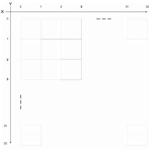
As shown in Figure 5.4.1, in 3DStreamer, we divide the world into 32 × 32 patches so that each patch can be stored, downloaded, and rendered independently. The terrain information for each patch is stored in its own data file, Terrain_y_x.dat, including all the data needed to render the patch, such as the height map, normal map, alpha blending textures, shadow map, terrain object information, and so on.

Figure 5.4.1. World consisting of 32×32 patches.

Tiles and Height Map

To generate the mesh for each terrain patch using the height map, we need to further divide each patch into tiles. As shown in Figure 5.4.2, each patch is divided into 32×32 tiles. A tile has four vertices, thus we have 33×33 vertices per patch. To render a terrain with varying heights, we assign each vertex of a patch a height. Altogether, we will have 33×33 height values, which constitute the height map of the patch.

Figure 5.4.2. Patch consisting of 32×32 tiles.

To build a mesh for each patch, we simply render each tile with two triangles, as shown in Figure 5.4.3.

Figure 5.4.3. Patch consisting of 32×32 tiles.

To build a 3D height map, we need to map the above 2D mesh to 3D space. Here is the mapping between the 2D coordinate (x’, y’) we used above and its 3D world coordinates (x, y, z):

{x, y, z} ç {x’, height, -y’}

As shown in Figure 5.4.4, the x’ axis of the 2D coordinates becomes the X-axis of the 3D world coordinate. The opposite of y’ axis of the 2D coordinates becomes the Z-axis of the 3D world coordinate. The 3D y-coordinate is given by the height of the vertices from the height map.

Figure 5.4.4. A rendered patch consisting of 32×32 tiles.

Figure5.4.4 shows a few terrain patches rendered by 3DStreamer. Note that the entire terrain (32×32 patches) is located between the X-axis (x’ axis of 2D space) and –Z-axis (y’ axis of 2D space). This makes the traversal of tiles and patches very easy: Both start from zero.

To stitch the patches together seamlessly, the 33rd column of vertices of the patch (x’ , y’) is replicated to the first column of vertices of the patch (x’+1, y’). Similarly, the 33rd row of patch (x’, y’) is replicated to the first row of patch (x’, y’+1).

The following constants define the scale of the terrain and reveal the relationship among patches, tiles, and vertices.

#define TILES_PER_PATCH_X 32
#define TILES_PER_PATCH_Y 32
#define PATCHES_PER_TERRAIN_X 32
#define PATCHES_PER_TERRAIN_Y 32
#define TILES_PER_TERRAIN_X (TILES_PER_PATCH_X * PATCHES_PER_TERRAIN_X)
#define TILES_PER_TERRAIN_Y (TILES_PER_PATCH_Y * PATCHES_PER_TERRAIN_Y)
#define VERTICES_PER_TERRAIN_X (TILES_PER_TERRAIN_X + 1)
#define VERTICES_PER_TERRAIN_Y (TILES_PER_TERRAIN_Y + 1)

3DStreamer has a random terrain generator that will generate random terrain data and store it into two types of output files.

Terrain_y_x.dat: The terrain patch (x,y)
Terrain_BB.dat: The bounding boxes for all patches

The reason that we need Terrain_BB.dat is for collision detection before the patches are loaded. To keep the avatar on the ground, even for patches not loaded, we need to be able to perform a rough collision detection using the patch’s bounding box (BB). Also, the BB enables us to perform a rough view frustum culling before the detailed mesh information of the patches is streamed over.

In a commercial MMO, the terrain data is usually handcrafted by a designer and artist to create a visually appealing environment. For demo and research purposes, though, it is convenient to generate an arbitrary large terrain procedurally and use it to stress the streaming engine.

Here is the process of how to generate random terrain data and deploy it using 3DStreamer.

Now we can run 3DStreamer in client mode to stream the above data from the HTTP server and render the terrain incrementally based on a user’s input. In production projects, though, you probably won’t use procedurally generated terrain with streaming because it’s much cheaper to send the seed parameters of the procedure instead of the output data of the procedure.

As described earlier, we will have a per-patch height map. From the height map, we’ll build the mesh for each patch as in the following code.

CreateMesh(int patch_x, int patch_y)
{
 TERRAINVertex* vertex = 0;
  D3DXCreateMeshFVF ( nrTri, nrVert, D3DXMESH_MANAGED,
                  TERRAINVertex::FVF, m_pDevice, &m_pMesh);
  m_pMesh->LockVertexBuffer(0,(void**)&vertex);
    for(int y = patch_y * TILES_PER_PATCH_Y, y0 = 0;
           y <= (patch_y+1) * TILES_PER_PATCH_Y;
           y++, y0++)
  for(int  x = patch_x * TILES_PER_PATCH_X, x0 = 0;
           x<= (patch_x+1) * TILES_PER_PATCH_X;
           x++, x0++)

   {
     int height = GetHeight(x, y);
     D3DXVECTOR3 pos = D3DXVECTOR3(x, height, -y);
     // Alpha UV stretches across the entire terrain in range [0, 1)
     D3DXVECTOR2 alphaUV = D3DXVECTOR2(x / VERTICES_PER_TERRAIN_X,
                                       y / VERTICES_PER_TERRAIN_Y);

     // Color UV repeats every 10 tiles
     D3DXVECTOR2 colorUV = alphaUV * TILES_PER_TERRAIN_X / 10.0f;
     vertex[z0 * (width + 1) + x0] =
            TERRAINVertex(pos, GetNormal(x, z), alphaUV, colorUV);
     // Update BBox of the patch
 }
m_pMesh->UnlockVertexBuffer();
…

}

First, we create a D3D mesh using the D3DXCreateMeshFVF API. Then we lock the mesh’s vertex buffer and fill it up with vertex information. For each tile (x,y) of the patch (patch_x, patch_y), we retrieve its height from the height map and build the position vector as (x, height, -y).

Next, we set up two sets of texture coordinates—colorUV for sampling texels from the terrain textures and alphaUV for sampling the alpha blending values of the terrain textures. We’ll discuss more about alpha blending in the next section. Then we calculate the normals of each vertex based on the height map. Note that we don’t want to only store the position vectors at the server and re-generate normals at the client, because normals on the patch border depend on the height from multiple patches. Since we need each patch to be independently renderable, it’s better that we store pre-computed normals with the patch data itself. During the process of adding vertices, we update the BBox of the patch and store it in the patch as well. The total size of vertex data of our demo terrain is about 40 bytes * (32 * 32) ^ 2 = 40 MB.

With the mesh set up for each patch, we’ll be able to render a wireframe terrain as shown in Figure 5.4.4. To give the terrain a more realistic look, we need to draw multiple types of textures on top of the mesh to represent different terrain features (for example, dirt, grass, and stone). Three common methods exist for multi-texturing terrain.

Alpha Blending Multi-Layer Textures

A better way to do this is to assign each texture to its own layer, create an alpha channel for each layer, and use a pixel shader to blend the textures. For example, we have three texture layers (dirt, grass, stone) in 3DStreamer and one alpha texture with three channels corresponding to the three layers. For each vertex, we can independently control whether it’s dirt, grass, or stone. This way, we will not have the obvious zigzag border between different textures because textures are assigned at the vertex level, not at the tile level. With per-tile texturing, two triangles of the same tiles are always assigned to the same texture, thus we’ll have the shape of the tile show up at the border between different texture areas. With alpha-blended multi-textures, the triangle that crosses the border of different textures will have different textures assigned to different vertices. Thus, the color of pixels inside the triangle will be interpolated based on samples from different textures.

As a result, we will have a tile-wide blending zone between different textures, which eliminates the clear zigzag border line. To further smooth the texture transition, we can broaden the blending zone by assigning partial textures to the vertex at the border. For example, instead of assigning a vertex with entirely dirt, grass, or stone, we can assign a vertex with 50 percent dirt and 50 percent grass if it is at the border.

The following code shows how we create a single alpha texture with three channels used to blend three layers of textures. We assign each vertex a texture type (dirt, grass, or stone) procedurally. We also apply a smoothing filter to the alpha texture so that alpha at the border transitions slower.

D3DXCreateTexture(pDevice, VERTICES_PER_TERRAIN_X, VERTICES_PER_TERRAIN_Y,
1, D3DUSAGE_DYNAMIC, D3DFMT_A8R8G8B8, D3DPOOL_DEFAULT, pAlphaMap);

 D3DLOCKED_RECT sRect;
(*pAlphaMap)->LockRect(0, &sRect, NULL, NULL);
BYTE *bytes = (BYTE*)sRect.pBits;

for(int i = 0;i < numOfTextures; i++)
  for(int y = 0; y < VERTICES_PER_TERRAIN_Y; y++)
  {
    for(int x = 0; x < VERTICES_PER_TERRAIN_X; x++)
    {
        TerrainTile *tile = GetTile(x,y);
       // Apply a filter to smooth the border among different tile types
        int intensity = 0;
        // tile->m_type has procedually generated texture types
        if(tile->m_type == i) ++intensity;
        tile = GetTile(x - 1, y);
        if(tile->m_type == i) ++intensity;
        tile = GetTile(x , y - 1);
        if(tile->m_type == i) ++intensity;
        tile = GetTile(x + 1, y);
        if(tile->m_type == i) ++intensity;
         tile = GetTile(x , y + 1);
         if(tile->m_type == i) ++intensity;
         bytes[y * sRect.Pitch + x * 4 + i] = 255 * intensity / 5;
       }
    }
(*pAlphaMap)->UnlockRect(0);

Figure 5.4.5 shows the effect of alpha blending of three different textures (dirt, grass, stone) rendered by 3DStreamer. As you can see, the transition from one to another is smooth. The total size of our terrain’s alpha-blending data is about 3 bytes * (32 * 32) ^ 2 = 3 MB.

Figure 5.4.5. Multi-texturing.

To create a dynamic 3D terrain, we need to draw shadows of the mountains. We can either calculate the shadow dynamically based on the direction of the light source or pre-calculate a shadow map based on a preset light source. The latter approach is much faster because it does not require CPU cycles at run time. Basically, we build a per-vertex shadow texture that covers the entire terrain. Each shadow texel represents whether the vertex is in shadow. We can determine whether a vertex is in shadow by creating a ray from the terrain vertex to the light source and test whether the ray intersects with the terrain mesh. If there is intersection, the vertex is in shadow, and it will have a texel value of 128 in the shadow map. Otherwise, it is outside shadow and has a texel value 255. We can then use a pixel shader to blend in the shadow by multiplying the shadow texel with the original pixel.

Figure 5.4.6 shows the effect of static shadow when the light source is preset at the left-hand side. The cost of storing the shadow texture of our terrain is not much—only 1 byte * (32 * 32) ^ 2 = 1 MB for the entire terrain.

Figure 5.4.6. Shadow.

Without any objects, the terrain looks boring. Thus, 3DStreamer adds two types of terrain objects (stones and trees) to the terrain. The mesh of each terrain object is stored in a .X file and loaded during startup. We are not streaming the .X files in 3DStreamer because there are only two of them. In a game where a lot of unique terrain objects are used, we should stream the model files of terrain objects as well.

To place terrain objects on top of terrain, we can use the terrain generator to randomly pick one of the object types and place it at a random tile with random orientation with a random size. We need to save the terrain objects’ placement information with the per-patch terrain data in order to redraw the objects at the client side. The following code fragment is an example of writing terrain object placement information to the disk for each tile during terrain generation.

OBJECT *object = tile->m_pObject;
If (object)
{
  out.write((char*)&object->m_type, sizeof(object->m_type));
  out.write((char*)&object->m_meshInstance.m_pos,
sizeof(object->m_meshInstance.m_pos));
  out.write((char*)&object->m_meshInstance.m_rot,
sizeof(object->m_meshInstance.m_rot));
  out.write((char*)&object->m_meshInstance.m_sca,
sizeof(object->m_meshInstance.m_sca));
} else
{
      OBJECTTYPE otype = OBJ_NONE;
      out.write((char*)&otype, sizeof(otype)
}

Assuming 20 percent of tiles have objects on them, the disk space taken by terrain objects’ placement information is about (4 B+12 B * 3) * (32 * 32)^2 * 20% = 8 MB.

Based on discussion in previous sections, our experiment terrain used in 3DStreamer consists of 32×32 patches and about one million tiles. Altogether, this takes about 60 MB of disk space to store. Here is a rough breakdown of the sizes of various components of the terrain data.

As shown in the Figure 5.4.7, it is a big terrain that takes a broadband user of 1-Mbps bandwidth 480 seconds (8 minutes) to download the complete data set. Thus, without streaming we cannot start rendering the terrain for eight minutes! With streaming we can start rendering the terrain in just a few seconds, and we will continuously stream the terrain patches the avatar interacts with over the network to the client.

Figure 5.4.7. Big terrain.

Streaming is a progressive data transfer and rendering technology that enables a “short wait” and “high-quality” content experience. The 3D streaming discussed here targets streaming over the network. However, the basic concepts and technique works for streaming from the disk as well. Disk streaming can be very convenient for debugging or research purposes (for example, if you don’t have an HTTP server set up, you can run 3DStreamer with data stored on a local disk, too). We want to build a data storage abstraction layer that allows us to source 3D terrain data from both the local disk and a remote file server. 3DStreamer defined a FileObject class for this purpose.

// Asynchronous File Read Interface for local disk read and remote HTTP read
class FileObject
{
public:
      FileObject(const char* path, int bufSize);
      ~FileObject();
      // Schedule the file object to be loaded
      void Enqueue(FileQueue::QueueType priority);
      // Wait until the file object is loaded
      void Wait();
      // Read data sequentially out of an object after it is loaded
      void Read(char* buf, int bytesToRead);
      virtual void Load(LeakyBucket* bucket) = 0;
};

FileObject provides an asynchronous file-loading interface consisting of the following public methods:

This is the main interface between the game’s prefetching algorithm and the underlying multi-queue asynchronous file read engine. The preloading algorithm will Enqueue() to queue a file object for downloading at the specified priority. The render will call Wait() to wait for critical data if necessary. We should avoid blocking the render thread as much as possible to avoid visual lag. Currently 3DStreamer only calls Wait() for loading the BB data at the beginning. The design goal of the prefetching algorithm is to minimize the wait time for the render loop. Ideally, the prefetching algorithm should have requested the right piece of content in advance, and the renderer will always have the data it needs and never need to block. When a file object is downloaded to the client, the render loop calls Read() to de-serialize the content from the file buffer to the 3D rendering buffers for rendering.

Behind the scene, the FileObject will interact with the FileQueueManager to add itself to one of the four queues with different priorities, as shown in Figure 5.4.8. The FileQueueReadThread will continuously dequeue FileObjects from the FileQueues according to the priority of the queues and invoke the FileObject::Load() virtual method to perform the actual download from the data source. We define the pure virtual method Load() as an interface to source specific downloading algorithms.

Figure 5.4.8. FileObject and FileQueue.

Both HTTPObject and DiskObject are derived from FileObject, and they encapsulate details of downloading a file object from the specific data source. They both implement the FileObject::Load() interface. So when FileQueueThread invokes the FileObject::Load(), the corresponding Load method of HTTPObject or DiskObject will take care of the data source–specific file downloading. Thus, FileObject hides the data source (protocol)–specific downloading details from the remainder of the system, which makes the asynchronous loading design agnostic to data source.

To fulfill the “low wait time” goal of game streaming, we need to achieve the following as much as possible:

The render loop does not block for streaming.

This translates into two requirements:

To fulfill the “high quality” goal for game streaming, we need to achieve the following requirements:

We will discuss the first three requirements here and leave the last requirement to later in this gem.

To support asynchronous loading (the first requirement), the render thread only enqueues a loading request to one of the prefetching queues via FileQueueManager and never blocks on loading. The FileQueueReadThread is a dedicated file download thread, and it dequeues a request from one of the four queues and executes it. FileQueueReadThread follows a strict priority model when walking through the priority queues. It starts with priority 0 and only moves to the next priority when the queue for the current priority is empty. After it dequeues a request, it will invoke the transport protocol–specific Load method to download the FileObject from the corresponding data source. (Refer to the “Transport Protocol” section for transport details.) At the end of the Load function, when data is read into memory of the client, the FileObject::m_Loaded is marked as true.

The third requirement is to react to players’ input promptly. Our multi-priority asynchronous queueing system supports on-the-fly cancel and requeue. At each frame, we will reevaluate the player’s area of interest, adjust the priorities of download requests, and move them across queues if necessary. To support the second requirement, the render loop will do the following: For patches in the viewing frustum and already submitted to DirectX (p->m_loaded is TRUE), we render them directly. For patches not submitted yet but already loaded to the file buffer (p->m_fileObject->m_loaded is TRUE), we call PuntPatchToGPU() to fill vertex/index/texture buffers with the data and then render the patches.

void TERRAIN::Render(CAMERA &camera)
{
  …
  for (int y = 0; y < m_numPatches.y; y++)
   for (int x = 0; x < m_numPatches.x; x++)
   {
    PATCH* p = m_patches[y * m_numPatches.x + x];
    if(!camera.Cull(p->m_BBox))
     {
       if (p->m_loaded)
          p->Render();
       if (p->m_fileObject && p->m_fileObject->m_loaded)
       {
          PuntPatchToGPU(p);
          p->Render();
       }
     }
   }
 …
}

With the above multi-priority asynchronous queueing system, we can load patches asynchronously with differentiated priority. The dedicated FileQueueReadThread thread decouples the file downloading from the video rendering in the main thread. As a result, video will never be frozen due to the lag in the streaming system. The worst case that could happen here is we walk onto a patch that is still being downloaded. This should rarely happen if our predictive loading algorithm works properly and we are within our tested and expected bandwidth amount. We did have a safety net designed in this case, which is the per-patch bounding box data we loaded during startup. We will simply use the BB of the patch for collision detection between the avatar and the terrain. So even in the worst case, the avatar will not fall under the terrain and die—phew!

We will use HTTP 1.1 as the transport protocol that supports persistent connections. Thus, all the requests from the same 3DStreamer client will be sent to the server via the same TCP connection. This saves us connection establishment and teardown overhead for downloading each patch. Also, HTTP gives us the following benefits:

As described in the “Transport Protocol” section, the HTTP transport is supported via HTTPObject, whose primary work is to implement the FileObject::Load() interface. The framework is very easy to extend to support other protocols as well, when such need arises.

A leaky bucket–based bandwidth rate limiter becomes handy when we need to evaluate the performance of a game streaming engine. Say we want to see how the terrain rendering works at different bandwidth caps—2 Mbps, 1 Mbps, and 100 Kbps—and tune our predictive loading algorithms accordingly, or we want to use the local hard disk as a data source to simulate a 1-Mbps connection, but the real hard disk runs at 300 Mbps—how do we do this?

Leaky bucket is a widely used algorithm for implementing a rate limiter for any I/O channel, including disk and network.

The following function implements a simple leaky bucket model. m_fillRate is how fast download credits (1 byte per unit) are filled into the bucket and is essentially the bandwidth cap we want to enforce. The m_burstSize is the depth of the bucket and is essentially the maximum burst size the bucket can tolerate. Every time the bucket is negative on credits, it returns a positive value, which is how many milliseconds the caller needs to wait to regain the minimum credit level.

int LeakyBucket::Update( int bytesRcvd )
{
   ULONGLONG tick = GetTickCount64();
 int deltaMs = (int)(tick - m_tick);
 if (deltaMs > 0)
 {
 // Update the running average of the rate
  m_rate = 0.5*m_rate + 0.5*bytesRcvd*8/1024/deltaMs;
  m_tick = tick;
 }
 // Refill the bucket
  m_credits += m_fillRate * deltaMs * 1024 * 1024 / 1000 / 8;
  if (m_credits > m_burstSize)
    m_credits = m_burstSize;
   // Leak the bucket
  m_credits -= bytesRcvd;
 if (m_credits >= 0)
   return 0;
 else
   return (-m_credits) * 8 * 1000 / (1024 * 1024) / m_fillRate;
}

This is the HTTP downloading code that invokes the leaky bucket for rate limiting.

void HttpObject::Load(LeakyBucket* bucket)
{
  …
  InternetReadFile(hRequest, buffer, m_bufferSize, &bytesRead);
  int ms = bucket->Update(bytesRead);
  if (ms)
     Sleep(ms);
  …
}

Figure 5.4.9 shows a scenario where we set the rate limiter to 1 Mbps to run a terrain walking test in 3DStreamer. The bandwidth we displayed is the actual bandwidth the 3DStreamer used, and it should be governed under 1 Mbps within the burst tolerance. Also, it shows how many file objects are in each priority queue. Since we are running fast with a relatively low bandwidth cap, there are some patches being downloaded in the four queues, including one critical patch close to the camera.

Figure 5.4.9. Bandwidth and prefetch queues.

The camera controls what the players see in the virtual world and how they see it. To minimize visual lag caused by streaming, it is crucial that the prefetching algorithm understands camera controls and synchronizes with the camera state.

A camera in the 3D rendering pipeline is defined by three vectors:

Some common camera controls supported by 3D games are:

3DStreamer supports all three controls. And the way we control the camera impacts the implementation of the predictive loading algorithm, as you can see next.

When do we need a patch of terrain to be loaded? When it is needed. We will present a few ways to calculate when the patches are needed in the following sections and compare them.

Probability-Based Distance Function

An avatar can move from its current location to the destination patch in different ways. For example:

1. Walk forward one patch and left shift one patch.

2. Turn left 45 degrees and walk forward 1.4 patch.

3. Turn right 45 degrees and left-shift 1.4 patch.

4. Take a portal connected to the patch directly.

5. Take a mount, turn left 45 degrees, and ride forward 1.4 patch.

I intentionally chose the word “way” instead of “path.” In order to use a length of the path as a distance function, the avatar must walk to the destination on the terrain at a constant speed. In reality, there are different ways and different speeds for the avatar to get to the patch, and they may or may not involve walking on the terrain. Also, the distance cannot be measured by the physical length of the route the avatar takes to get to the patch in some cases (such as teleporting). A more universal unit to measure the distance of different ways is the time it takes the avatar to get there. With the above example, the time it takes the avatar to get to the destination is:

1. Assuming forward speed is 0.2 patch/second and left-shift speed is 0.1 patch/second, it takes the avatar 5 + 10 = 15 seconds to get there.

2. Assuming the turning speed is 45 degrees/second, it takes the avatar 1 + 7 = 8 seconds to get there.

3. It takes 1 + 14 = 15 seconds to get there.

4. Assuming the portal takes 5 seconds to start and 5 seconds in transit, it takes 10 seconds to get there.

5. Assuming the mount turns and moves two times as fast, it takes 8 / 2 = 4 seconds to get there.

Let’s say we know that the probabilities of the avatar to use the aforementioned ways to get to patch p are: 0.2, 0.6, 0.0 (it’s kind of brain-dead to do 3), 0.1, and 0.1, respectively.

The probability-based distance D(p) will then be given by: 15 * 0.2 + 8 * 0.6 + 10 * 0.1 + 4 * 0.1 = 3 + 4.8 + 1 + 0.4 = 9.2 seconds.

Thus, the probability-based distance function can be written as:

where p(i) is the probability of the avatar taking way i to get to patch p, and t(i) is the time it takes to get to p using way i.

As you can see, the power of this probability-based distance function is that it can be expanded to an extent as sophisticated as we want depending on how many factors we want to include to guide the predictive loading algorithm. For a game where we want to consider all kinds of combinations of moving options for an avatar, we can model the moving behavior of the avatar statistically in real time and feed statistics back to the above formula to have very accurate predictive loading. At the same time, we can simplify the above formula as much as we can to have a simple but still reasonably accurate predictive loading algorithm. In the 3DStreamer demo, we simplify the distance function as the following.

First, 3DStreamer does not support teleporting or mount, so options 4 and 5 are out of consideration. Second, as in most games, 3DStreamer defines the speeds for left/right shifting and moving backward at a much lower value than the speed of moving forward. From the user experience point of view, it’s more intuitive for the player to move forward anyway. So in 3DStreamer, we assume that the probability of an avatar using the “turn and go forward” way is 100 percent. With this assumption, the distance function is reduced to:

D(p) = rotation time + moving time= alpha / w + d / v.

Alpha is the horizontal angle the camera needs to rotate to look at the center of p directly. w is the angular velocity for rotating the camera. d is the straight-line distance between the center of p and the camera. v is the forward-moving speed of the avatar.

The following code fragment shows the implementation of the predictive loading in 3DStreamer based on the simplified distance function.

D3DXVECTOR2 patchPos(((float)mr.left + mr.right) / 2, ((float)mr.top +
mr.bottom) / 2);
D3DXVECTOR2 eyePos(camera.Eye().x, - camera.Eye().z);
D3DXVECTOR2 eyeToPatch = patchPos - eyePos;
float patchAngle = atan2f(eyeToPatch.y, eyeToPatch.x); // [-Pi, +Pi]

// Calculate rotation distance and rotation time
float angleDelta = abs(patchAngle - camera.Alpha());
if (angleDelta > D3DX_PI)
    angleDelta = 2 * D3DX_PI - angleDelta;

float rotationTime = angleDelta / camera.AngularVelocity();

// Calculate linear distance and movement time
float distance = D3DXVec2Length(&eyeToPatch);
float linearTime = distance / camera.Velocity();

float totalTime = rotationTime + linearTime;
float patchTraverseTime = TILES_PER_PATCH_X / camera.Velocity();
if (totalTime < 2 * patchTraverseTime)
      RequestTerrainPatch(patch_x, patch_y, FileQueue::QUEUE_CRITICAL);
else if (totalTime < 4 * patchTraverseTime)
      RequestTerrainPatch(patch_x, patch_y, FileQueue::QUEUE_HIGH);
else if (totalTime < 6 * patchTraverseTime)
      RequestTerrainPatch(patch_x, patch_y, FileQueue::QUEUE_MEDIUM);
else if (totalTime < 8 * patchTraverseTime)
      RequestTerrainPatch(patch_x, patch_y, FileQueue::QUEUE_LOW);
  else
  {
        If (patch->m_loaded)
             patch->Unload();
        else if (patch->m_fileObject->GetQueue() != FileQueue::QUEUE_NONE)
           CancelTerrainPatch(patch);
}

For each frame, we reevaluate the distance function of each patch and move the patch to the proper priority queue accordingly. The ability to dynamically move file prefetching requests across priorities is important. This will handle the case where an avatar makes a sharp turn and the high-priority patch in front of the avatar suddenly becomes less important. In an extreme case, a patch earlier in one of the priority queues could be downgraded so much that it’s canceled from the prefetching queues entirely.

Note that in the last case, where D(p) >= 8 * patchTraverseTime, we will process it differently depending on its current state.

• Already loaded. Unload the patch and free memory for mesh and terrain objects.

• Already in queue. Cancel it from the queue.

With this predictive loading algorithm, 3DStreamer can render a terrain of one million tiles at 800×600 resolution under 1-Mbps bandwidth pretty decently. At a speed of 15 tiles/second, we still get enough time to prefetch most nearby patches in the avatar’s viewing frustum, even though we make sharp turns.

Figure 5.4.10 shows what it looks like when we run the avatar around at 15 tiles/s with only 1-Mbps bandwidth to the HTTP streaming server. The mini-map shows which patches of the entire terrain have been preloaded, and the white box in the mini-map is the intersection of the viewing frustum with the ground. As you can see, the avatar is moving toward the upper-left corner of the map. As shown by “Prefetch Queues,” all the critical- and high-priority patches are loaded already, which corresponds to all the nearby patches in the viewing frustum plus patches to the side of and behind the player. The medium- and low-priority queues have 80 patches to download, which are mostly the faraway patches in front of the player.

Figure 5.4.10. Predictive loading under 1-Mbps bandwidth at 15 tiles/s.

Also note that the non-black area in the mini-map shows the current memory footprint of the terrain data. It is important that when we move the avatar around, we unload faraway patches from memory to create space for new patches. This way, we will maintain a constant memory footprint regardless of the size of the entire terrain, which is a tremendously important feature of a 3D streaming engine in order to scale up to an infinitely large virtual world.

3DStreamer.sln can be loaded and compiled with Visual Studio 2008 with DirectX November 2008 or newer. The data is staged to the Debug folder for debug build by default. In order to run a release build, you need to manually copy the data (data, models, shaders, textures) from the Debug folder to the Release folder.

Running the 3DStreamer with the following command will generate a random 32 × 32-patch terrain and save the data in the executable’s folder. It will take a while to complete. Alternatively, just use the pre-generated data in the DebugData folder on the CD-ROM.

3DStreamer -g

For HTTP streaming, upload the data (terrain_XX_YY.dat and terrain_BB.dat) to your HTTP server and use the -s= command line argument to specify the server’s host name and the -p= argument to specify the location of the data on the server.

For DISK streaming, simply give the data’s path as the -p= argument.

To run it in VS, please make sure to add $(OutDir) to the Working Directory of the project properties. Alternatively, you can run the executable from the executable folder directly. By default, 3DStreamer runs in DISK streaming mode with a default data path pointing to the executable folder.

To run it in HTTP streaming mode, you need to give the -s argument for the host name. For example, to stream the data from a server URL http://192.168.11.11/3dstreamer/32x32, just run it with the following command line:

3DStreamer -h -s=192.168.11.11 -p=3dstreamer32x32

Note that the trailing slash in the path is important. Otherwise, the client cannot construct the proper server URL.

You can also adjust the bandwidth cap (the default is 1 Mbps) with the -b= argument. For example, to run it in DISK streaming mode simulating a 2-Mbps link, just enter:

3DStreamer –b=2