
Dave Mark, Intrinsic Algorithm LLC
One of the challenges of creating deep, interesting behaviors in games and simulations is to enable our agents to select from a wide variety of actions while not abandoning completely deterministic systems. On the one hand, we want to step away from having very obvious if/then triggers or monotonous sequences of actions for our agents. On the other hand, the need for simple testing and debugging necessitates the avoidance of introducing random selection to our algorithms.
This gem shows how, through embracing the concept and deterministic techniques of chaos theory, we can achieve complex-looking behaviors that are reasonable yet not immediately predictable by the viewer. By citing examples from nature and science (such as weather) as well as the simple artificial simulations of cellular automation, the gem explains what causes chaotic-looking systems through purely deterministic rules. The gem then presents some sample, purely deterministic behavior systems that exhibit complex, observably unpredictable sequences of behavior. The gem concludes by explaining how these sorts of algorithms can be easily integrated into game AI and simulation models to generate deeper, more immersive behavior.
The game development industry often finds itself in a curious predicament with regard to randomness in games. Game developers rely heavily on deterministic systems. Programming is inherently a deterministic environment. Even looking only at the lowly if/then statement, it is obvious that computers themselves are most “comfortable” in a realm where there is a hard-coded relationship between cause and effect. Even non-binary systems, such as fuzzy state machines and response curves, could theoretically be reduced to a potentially infinite sequence of statements that state, “Given the value x, the one and only result is y.”
Game designers, programmers, and testers also feel comfortable with this technological bedrock. After all, in the course of designing, developing, and observing the complex algorithms and behaviors, they often have the need to be able to say, with certainty, “Given this set of parameters, this is what should happen.” Often the only metric of the success or failure of the development process we have is the question, “Is this action what we expected? If not, what went wrong?”
Game players, on the other hand, have a different perspective on the situation. The very factor that comforts the programmer—the knowledge that his program is doing exactly what he predicts—is the factor that can annoy the player…the program is doing exactly what he predicts. From the standpoint of the player, predictability in game characters can lead to repetitive, and therefore monotonous, gameplay.
The inclusion of randomness can be a powerful and effective tool to simulate the wide variety of choices that intelligent agents are inclined to make [Mark09]. Used correctly and limiting the application to the selection of behaviors that are reasonable for the NPC’s archetype, randomness can create deeper, more believable characters [Ellinger08]. While this approach provides a realistic depth of behavior that can be attractive to the game player, it is this same abandonment of a predictable environment that makes the analysis, testing, and debugging of behaviors more complicated. Complete unpredictability can also lead to player frustration, as they are unable to progress in the game by learning complex agent behavior. The only recourse that a programming staff has in controlling random behaviors is through tight selection of random seeds. In a dynamic environment, however, the juxtaposition of random selection of AI with the unpredictable nature of the player’s actions can lead to a combinatorial explosion of possible scenario-to-reaction mappings. This is often a situation that is an unwanted—or even unacceptable—risk or burden for a development staff.
The solution lies in questioning one of the premises in the above analysis—that is, that the experience of the players is improved through the inclusion of randomness in the decision models of the agent AI. While that statement may well be true, the premise in question is that the experience that the player has is based on the actual random number call in the code. The random number generation in the agent AI is merely a tool in a greater process. What is important is that the player cannot perceive excessive predictable regularity in the actions of the agent. As we shall discuss in this article, accomplishing the goal of unpredictability can exist without sacrificing the moment-by-moment logical determinism that developers need in order to confidently craft their agent code.
The central point of how and why this approach is viable can be illustrated simply by analyzing the term chaos theory. The word chaos is defined as “a state of utter confusion or disorder; a total lack of organization or order.” This is also how we tend to use it in general speech. By stating that there is no organization or order to a system, we imply randomness. However, chaos theory deals entirely within the realm of purely deterministic systems; there is no randomness involved. In this sense, the idea of chaos is more aligned with the idea of “extremely complex information” than with the absence of order. To the point of this article, because the information is so complex, we observers are unable to adequately perceive the complexity of the interactions. Given a momentary initial state (the input), we fail to determine the rule set that was in effect that led to the next momentary state (the output).
Our inability to perceive order falls into two general categories. First, we are often limited by flawed perception of information. This occurs by not perceiving the existence of relevant information and not perceiving relevant information with great enough accuracy to determine the ultimate effect of the information on the system.
The second failure is to adequately perceive and understand the relationships that define the systems. Even with perfect perception of information, if we are not aware of how that information interacts, we will not be able to understand the dynamics of the system. We may not perceive a relationship in its entirety or we may not be clear on the exact magnitude that a relationship has. For example, while we may realize that A and B are related in some way, we may not know exactly what the details of that relationship are.
Chaos theory is based largely on the first of these two categories—the inability to perceive the accuracy of the information. In 1873, the Scottish theoretical physicist and mathematician James Clerk Maxwell hypothesized that there are classes of phenomena affected by “influences whose physical magnitude is too small to be taken account of by a finite being, [but which] may produce results of the highest importance.”
As prophetic as this speculation is, it was the French mathematician Henri Poincaré, considered by some to be the father of chaos theory, who put it to more formal study in his examination of the “three-body problem” in 1887. Despite inventing an entirely new branch of mathematics, algebraic topology, to tackle the problem, he never completely succeeded. What he found in the process, however, was profound in its own right. He summed up his findings as follows:
If we knew exactly the laws of nature and the situation of the univ erse at the initial moment, we could predict exactly the situation of the same univ erse at a succeeding moment. But even if it were the case that the natural laws had no longer any secret for us, we could still know the situation approximately. If that enabled us to predict the succeeding situation with the same approximation, that is all we require, and we should say that the phenomenon had been predicted, that it is governed by the laws. But [it] is not always so; it may happen that small differences in the initial conditions produce very great ones in the final phenomena. A small error in the former will produce an enormous error in the later. Prediction becomes impossible…. [Wikipedia09]
This concept eventually led to what is popularly referred to as the butterfly effect. The origin of the term is somewhat nebulous, but it is most often linked to the work of Edward Lorenz. In 1961, Lorenz was working on the issue of weather prediction using a large computer. Due to logistics, he had to terminate a particularly long run of processing midway through. In order to resume the calculations at a later time, he made a note of all the relevant variables in the registers. When it was time to continue the process, he re-entered the values that he had recorded previously. Rather than reenter one value as 0.506127, he simply entered 0.506. Eventually, the complex simulation diverged significantly from what he had predicted. He later determined that the removal of 0.000127 from the data was what had dramatically changed the course of the dynamic system—in this case, resulting in a dramatically different weather system. In 1963, he wrote of his findings in a paper for the New York Academy of Sciences, noting that, “One meteorologist remarked that if the theory were correct, one flap of a seagull’s wings could change the course of weather forever.” (He later substituted “butterfly” for “seagull” for poetic effect.)
Despite being an inherently deterministic environment, much of the problem with predicting weather lies in the size of the scope. Certainly, it is too much to ask scientists to predict on which city blocks rain will fall and on which it will not during an isolated shower. However, even predicting the single broad path of a large, seemingly well-organized storm system, such as a hurricane, baffles current technology. Even without accounting for the intensity of the storm as a whole, much less the individual bands of rain and wind, the various forecasts of simply the path of the eye of the hurricane that the different prediction algorithms churn out lay out like the strings of a discarded tassel. That these mathematical models all process the same information in such widely divergent ways speaks to the complexity of the problem.
Thankfully, the mathematical error issue is not much of a factor in the closed system of a computer game. We do not have to worry about errors in initial observations of the world, because our modeling system is actually a part of the world. If we restart the model from the same initial point, we can guarantee that, unlike Lorenz’ misfortune, we won’t have an error of 0.000127 to send our calculations spinning off wildly into the solar system. (Interestingly, in our quest for randomness, we can build a system that relies on a truly random seed to provide interesting variation—the player.) Additionally, we don’t have to worry about differences in mathematical calculation on any given run. All other things being equal (for example, processor type), a given combination of formula and input will always yield the same output. These two factors are important in constructing a reliable deterministic system that is entirely under our control.
As mentioned earlier, the second reason why people mistake deterministic chaos for randomness is that we often lack the ability to perceive or realize the relationships between entities in a system. In fact, we often are not aware of some of the entities at all. This was the case with the discovery of a phenomenon that eventually became known as Brownian motion. Although there had been observations of the seemingly random movement of particles before, the accepted genesis of this idea is the work of botanist Robert Brown in 1827. As he watched the microscopic inner workings of pollen grains, he observed minute “jittery” movement by vacuoles. Over time, the vacuoles would even seem to travel around their neighborhood in an “alive-looking” manner. Not having a convenient explanation for this motion, he assumed that pollen was “alive” and was, after the way of living things, moving of its own accord. He later repeated the experiments with dust, which ruled out the “alive” theory but did nothing to explain the motion of the particles.
The real reason for the motion of the vacuoles was due to the molecular and atomic level vibrations due to heat. Each atom in the neighborhood of the target vibrates on its own pattern and schedule, with each vibration nudging both the target and other adjacent atoms slightly. The combination of many atoms doing so in myriad directions and amounts provides a staggering level of complexity. While completely deterministic from one moment to the next—that is, “A will nudge B n distance in d direction”— the combinatorial explosion of interconnected factors goes well beyond the paltry scope of Poincaré’s three-body problem.
The problem that Brown had was that he could not perceive the existence of the atoms buffeting the visible grains. What’s more, even when the existence of those atoms is known (and more to the point, once the heat-induced vibration of molecules is understood), there is no way that anyone can know what that relationship between cause and effect is from moment to moment. We only know that there will be an effect.
This speaks to the second of the reasons we listed earlier—that we often lack the ability to perceive or realize the relationships between entities in a system. This effect is easier for us to take advantage of in order to accomplish our goal. By incorporating connections between agents and world data that are beyond the ability of the player to adequately perceive, we can generate purely deterministic cause/effect chains that look either random or at least reasonably unpredictable.
One well-known example bed for purely deterministic environments is the world of cellular automata. Accordingly, one of the most well-known examples of cellular automata is Conway’s Game of Life. Conway’s creation (because the term “game” is probably pushing things a little) started as an attempt to boil down John von Neumann’s theories of self-replicating Turing machines. What spilled out of his project was an interesting vantage point on emergent behavior and, more to the point of this gem, the appearance of seemingly coordinated, logical behavior. Using Conway’s Life as an example, we will show how applying simple, deterministic rules produce this seemingly random behavior.
The environment for Life is a square grid of cells. A cell can be either on or off. Its state in any given time slice is based on the states of the eight cells in its immediate neighborhood. The number of possible combinations of the cells in the local neighborhood is 28 or 256. (If you account for mirroring or rotation of the state space, the actual number of unique arrangements is somewhat smaller.) The reason that the Game of Life is easy for us to digest is its brevity and simplicity, however. We do not care about the orientation of the live neighbors, but only a sum of how many are alive at that moment. The only rules that are in effect are:
Any live cell with two or three live neighbors lives on to the next generation.
Any live cell with fewer than two live neighbors dies (loneliness/starvation).
Any live cell with more than three live neighbors dies (overcrowding).
Any dead cell with exactly three live neighbors becomes a live cell (birth).
Figure 3.7.1 shows a very simple example of these rules in action. In the initial grid, there are three “live” cells shown in black. Additionally, each cell contains a number showing how many neighbors that cell currently has. Note that two of the “dead” cells (shown in gray) have three neighbors, which, according to Rule 4 above, means they will become alive in the next iteration. The other dead cells have zero, one, or two neighbors, meaning they will remain at a status quo (in other words, dead) for the next round. The center “live” cell has two neighbors, which, according to Rule 1 above, allows it to continue living. On the other hand, the two end cells have only a single live neighbor (the center cell) and will therefore die of starvation the next round. The results are shown on the right of Figure 3.7.1. Two of the prior cells are now dead (shown in gray), and two new cells have been born to join the single surviving cell.
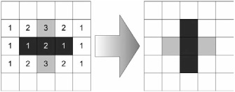
Figure 3.7.1. A simple example of the rule set in Conway’s Game of Life. In this case, a two-step repeating figure called a blinker is generated by the three boxes.
Interestingly, this pattern repeats such that the next iteration will be identical to the first (a horizontal line), and so on. This is one of the many stable or tightly repeating patterns that can be found in Life. Specifically, this one is commonly called a blinker.
Figure 3.7.2 shows another, slightly more involved example. The numbers in the initial frame make it easier to understand why the results are there. Even without the numbers, however, the relationships between the initial state and the subsequent one are relatively easy to discern on this small scale.

While the rule set seems simple and intuitive enough, when placed on a larger scale and run over time, the “behavior” of the entire “colony” of cells starts to look random. This is due to the overwhelming number of interactions that we perceive at any one moment. Looking at the four panels of Figure 3.7.3, it is difficult for us to intuitively predict what would have happened next except for either in the most general sense (for example, that solid blob in the middle is too crowded and will likely collapse) or in regard to very specific subsets of the whole (for example, that is a blinker in the lower-left corner).
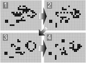
Figure 3.7.3. When taken as a whole, the simple cells in Life take on a variety of complex-looking behaviors. While each cell’s state is purely deterministic, it is difficult for the human mind to quickly predict what the next overall image will look like.
Interestingly, it is this very combination of “reasonable” expectations with not knowing exactly what is going to appear next that gives depth to Conway’s simulation. Over time, one develops a sense of familiarity with the generalized feel of the simulation. For example, we can expect that overcrowded sections will collapse under their own weight, and isolated pockets will die off or stagnate. We also recognize how certain static or repeating features will persist until they are interfered with—even slightly— by an outside influence. Still, the casual observer will still perceive the unfolding (and seemingly complex) action as being somewhat random…or at least undirected. Short of pausing to analyze every cell on every frame, the underlying strictly rule-based engine goes unnoticed.
On the other hand, from the standpoint of the designer and tester, this simulation model is elegantly simplistic. The very fact that you can pause the simulation and confirm that each cell is behaving properly is a boon. For any given cell at any stage, it is a trivial problem to confirm that the resulting state change is performing exactly as designed.
What sets Conway’s Life apart from many game scenarios is not the complexity of the rule set, but rather the depth of it. On its own, the process of passing the sum of eight binary inputs through four rules to receive a new binary state does not seem terribly complex. When we compare it to what a typical AI entity in a game may use as its decision model, we realize that it is actually a relatively robust model.
For instance, imagine a very simple AI agent in a first-person shooter game (see Figure 3.7.4). It may take into account the distance to the player and the direction in which the player lies. When the player enters a specified range, the NPC “wakes up,” turns, and moves toward the player. There is one input state—distance—and two output states: “idle” and “move toward player.” While this seems extraordinarily simple, as recently as 10 to 15 years ago, this was still common for enemy AI. Needless to say, the threshold and resultant behavior were easy to discern over time. Players could perceive both the cause and the effect with very little difficulty. Likewise, designers and programmers could test this behavior with something as simple as an onscreen distance counter. At this point, there is very little divergence between the simplicity for the player and the simplicity for the programmer.
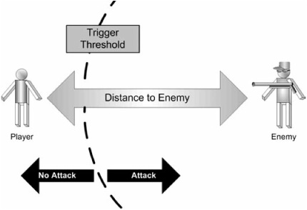
Figure 3.7.4. If there is only one criterion in a decision model, it is relatively simple for the player to determine not only what the criterion is, but what the critical threshold value is for that criterion to trigger the behavior.
If we were to add a second criterion to the decision, the situation does not necessarily become much more complicated. For example, we could add a criterion stating that the agent will only attack the player when he is in range and carrying a weapon. This is an intuitively sound addition and is likely something that the player will quickly understand. On the other hand, this also means that the enemy is again rigidly predictable.
Other factors can be added to a decision model, however, which could obscure the point at which a behavior change should occur. Even the addition of other binary factors (such as the states of the cells in Life) can complicate things quickly for the observer if they aren’t intuitively obvious. For instance, imagine that the rule for attacking the player was no longer “if the distance from player to enemy < n” but rather “if the player’s distance to two enemies < n” (see Figure 3.7.5). As the player approaches the first enemy, there would be no reaction from that first enemy until a second enemy is within range as well. While this may seem like a contrived rule, it stresses an important point. The player will most certainly be interested in the actions of the first enemy and will not easily recognize that its reaction was ultimately based on the distance to the second enemy.

Figure 3.7.5. The inclusion of a second criterion can obscure the threshold value for—or even the existence of—the first criterion. In this case, because the second enemy is included, the player is not attacked as he enters the normal decision radius of the first enemy.
The player may not be able to adequately determine what the trigger conditions are because we have masked the existence of the second criterion from the player. People assume that causes and effects are linked in some fashion. In this example, because there is no intuitive link between the player’s distance to the second enemy and the actions of the first, the player will be at a loss to determine when the first enemy will attack. The benefit of this approach is that the enemy no longer seems like it is acting strictly on the whims of the player. That is, the player is no longer deciding when he wants the enemy to attack—it is seemingly attacking on its own. This imparts an aura of unpredictability on the enemy, which, in essence, makes it seem more autonomous.
Of course, we programmers know that the agent is not truly autonomous but merely acting as a result of second criterion. In fact, this new rule set is almost as simple to monitor and test as it is to program in the first place. We have the benefit of knowing what the two rules are and how they interact—something that is somewhat opaque to the player.
As mentioned, the inclusion of the player’s distance to the second agent as a criterion for the decisions of the first agent is a little contrived. In fact, it has the potential for embarrassing error. If the second agent was far away, it is possible that the player could walk right up to the first one and not be inside the threshold radius of the second. In this case, the first agent would check his decision criteria and determine that the player was not in range of two people and, as a result, would not attack the player. This does not mean that there is a flaw in the use of more than one criterion for the decision—simply that there is a flaw in which criteria are being used in conjunction. In this case, the criterion that was based on the position of the second agent—and, more specifically, the player’s proximity to the second agent—was arbitrary. It was not directly related to the decision that the agent is making.
The solution to this is to include factors on which it is reasonable for an agent to base his decisions. In this example, the factors may include items such as:
Distance to player
Perceived threat (for example, visible weapon)
Agent’s health
Agent’s ammo
Agent’s alertness level
Player’s distance to sensitive location
We already covered the first two. The others are simply examples of information that could be considered relevant. For the last one, we could use the distance measurement from the player to a location such as a bomb detonator. If the player is too close to it, the agent will attack. This is different than the example with two agents above in that the distance to a detonator is presumably more relevant to the agent’s job than the player’s proximity to two separate agents.
While a number of the criteria listed previously could be expressed as continuous values, such as the agent’s health ranging from 0 to 100, for the sake of simplicity, they can also be reduced to Boolean values. We could rephrase “agent’s health” as “agent has low health,” for instance. If we define “low health” as a value below 25, we are now able to reduce that criterion to a Boolean value. The same could be done with “agent’s ammo.” This, of course, is very similar to what we did with the distance. We could assert that “if agent has less than 10 shots remaining,” then “agent has low ammo.”
What we have achieved with the above list could be summed up with the following pseudo-code query:
If  PlayerTooCloseToMe()
    or PlayerCloseToTarget()
    and WeaponVisible()
    and IAmHealthy()
    and IHaveEnoughAmmo()
    and IAmAlert())
    then Attack()
Even with these criteria, the number of possible configurations is 27 or 128. (Incidentally, the number of configurations of cells in Life is 28 or 256.) In our initial example, it would take only a short amount of time to determine the distance threshold at which the agent attacks. By the inclusion of so many relevant factors into the agent’s behavior model, the only way that any one threshold can be ascertained is with the inclusion of the caveat “all other things being equal.” Certainly in a dynamic environment, it is a difficult prospect to control for all variables simultaneously.
While having 128 possible configurations seems like a lot, it is not necessarily the number of possible configurations of data that will obscure the agent’s possible selection from the player. Much of the difficulty that a player would have in knowing exactly what reaction the agent will have is due to the fact that the player cannot perceive all the data. This is similar to the impasse at which Robert Brown found himself. He could not detect the actual underlying cause of the jitteriness of the pollen grains and dust particles. His observation, therefore, was that the motion was random yet reasonable; he perceived lifelike motion where there was no life.
A good way of illustrating this point is by working backward—that is, looking at the situation from the point of the player. If the agent’s behavior changes from one moment to the next, the player may not be able to determine which of the aforementioned factors crossed one of the defined thresholds to trigger the change. In some cases, this would be easy. For example, if the player draws his weapon and the agent attacks, the player can make the assertion that the weapon was the deciding factor. However, if the agent does not attack and, for instance, runs away instead, the player may not be able to determine whether it was due to the agent having low health or low ammo.
Similarly, if the player is moving near the agent with his weapon drawn, and the agent begins to attack, the player may not be able to ascertain whether it was his proximity to the agent, a secondary point (for example, a detonator), or a change in the agent’s alertness status that caused the transition to occur. Once combat is engaged and values such as health and ammo are changing regularly, the number of possible reasons for a change in behavior increases significantly.
Of course, this is the reason why it is important to use relevant information as part of your decision. If you use rational bases for your decisions, it makes it more likely that the decision can at least be understood after it happens. There is a big difference between predictability and understandability. The player may not know exactly when the agent is going to change behaviors, but he should be able to offer a reasonable guess as to why it happened.
From a development and testing standpoint, the important issue to note here is that this is still purely deterministic. There is no randomness included at all. A simple code trace or onscreen debug information would confirm the status of all seven of these criteria. When compared against the decision code, the developer can confirm whether the agents are operating as planned or, in the case that they are not, determine which of the criteria needs to be adjusted.
We can extend the aforementioned ideas to go beyond purely Boolean flags, however. By incorporating fuzzy values and appropriate systems to handle them, we could have more than one threshold value on any of the previous criteria. For instance, we could use the seven aforementioned factors to select from a variety of behaviors. Rather than simply determining whether the agent will attack the player, for example, we could include actions such as finding cover, running away, reloading, or calling for help. In order to do this, we could partition one or many of the factors into multiple zones.
For example, if we were to arrange two factors on two axes and determine a threshold across each, we would arrive at four distinct “zones” (see Figure 3.7.6, Panel 1). Each of these zones can be assigned to a behavior. In this case, using only two factors and two threshold values, we can arrive at four distinct behaviors. The more thresholds we insert, the more zones are created. Using our two-axis example, by increasing the threshold values from 1 to 3 in each direction, we increase the number of result spaces from 4 to 16 (see Figure 3.7.6, Panel 2).

Figure 3.7.6. As the number of logical partitions through axes is increased, the number of potential results increases exponentially as a factor of the number of axes involved. By combining the factors prior to partitioning (Panel 3), thresholds can be made more expressive.
We can visualize how this would affect behaviors if we imagine the values of our two factors moving independently along their respective axes. For example, imagine a data point located in Behavior G in Panel 2. If Factor 1’s value were to change, we could expect to see Behaviors F and H—and even E—depending on the amount of change in Factor 1. If Factor 2 were the only one changing, we could expect to see changes to Behaviors C, K, and O. If changes were occurring in only Factor 1 or 2, by observing the changes in behavior that occurred, we could eventually determine where those thresholds between behaviors are. However, if both factors were continually changing independent of each other, we now could possibly see any one of the 16 behaviors. This would make it significantly more difficult to exactly predict the cause-and-effect chain between factors and behaviors.
For instance, assume once again that we start with the data point in G. If we were witnessing a reduction in Factor 1, we may see a state change to B, C, F, J, or K. All of those states can be reached from G if Factor 1 is decreasing. What we would have to realize is that the ultimate state is decided by Factor 2 as well—for example, G→C could happen if Factor 1 was decreasing slowly and Factor 2 was increasing. Correspondingly, G→K could happen if Factor 1 was decreasing slowly and Factor 2 was decreasing. Naturally, similar extensions of logic apply to result states of B and J. The conclusion is, while we can make a general statement about where our data point may end up while Factor 1 is decreasing, we can’t know the eventual result state without also knowing the behavior of Factor 2.
The examples shown in Figure 3.7.6 only show two dimensions due the limitations of what can be shown on paper. Our decision model does not share those limitations, however. By using each potential factor in our decision model and defining one or more thresholds of meaning, we can create a complex state space of potential results.
As a measurement of how this expands the potential number of actions, we can compare the number of possible outcomes. When the system was composed of 7 Boolean values, we had 128 possible combinations of data. Even by simply partitioning each of the 7 inputs into 3 ranges rather than 2, the number of combinations becomes 37 or 2,187. These results could then be mapped to a startling array of behaviors. Of course, not all the result zones need to represent individual behaviors. Imagine mapping the 2,187 possible result spaces onto 30 different behaviors, for instance.
To further leverage the power of this system, we can step beyond the mentality of mapping a single value onto a series of states. Instead, we can use systems that can take multiple inputs in conjunction and select a state that is dependant on values of those multiple inputs.
For example, we may want our agent to consider a combination of its distance to the player and their own health. That is, the state of their own health becomes more important if the player is closer. The two endpoints of the “relevancy vector” of this decision would be between (“player far” + “perfect health”) and (“player near” + “zero health”). As either of those factors moves from one end to the other, it has less effect on the outcome than if both of these factors were moving simultaneously.
Figure 3.7.6, Panel 3 shows a two-dimensional visualization of this effect. In this case, the factors themselves are not partitioned. Instead, they remain continuous variables. When combined, however, they create a new directed axis in the state space— in this case shown by the combined shading. We can set a threshold across that new axis (dotted line) that can be used to determine where the behavior changes. Now, from the point of view of the player, he cannot determine at what point on Factor 1 the behavior changes without taking into account changes in Factor 2 as well.
Just as we did with single-axis-based thresholds, by determining one or more multi-axis threshold lines in an n-dimensional space, we partition our space into a variety of zones. By analyzing in which sections of the resulting partitioned space our current input data falls, we can select from multiple potential outputs. By combining values in this way, we can potentially arrive at more expressive outputs at any stage of our decision model.
Specific techniques for accomplishing and managing this sort of decision complexity can be found elsewhere [Mark08]. The methods that we use to arrive at the resulting values are not the focus here, however. The important part is that we are doing all of this in a purely deterministic fashion—that is, we could verify that any given combination of factors is mapped to the appropriate action. While there is still no random factor being included in these calculations, the dizzying number of potential combinations provides for reasonable-looking, yet not inherently predictable results.
To sum up, while our desire as game developers may be to express a variety of reasonable-looking but slightly unpredictable behaviors, we do not have to resort to randomness in order to generate that effect. By including more than one or two simple, easily perceivable criteria in our decision models, we can begin to obscure the workings of that model from the player, yet leave it perfectly exposed and understandable to the programmer and even the design team. However, in order to avoid the potential for arbitrary-looking decisions by our agents, we must be careful to select criteria that are relevant to the decision being made. In this way we are also providing deeper, more realistic-looking, and potentially more immersive behaviors for our agents.