CHAPTER 16

Compositing

COMPOSITING IS A POST-PRODUCTION process critical to the workflow of many artists creating complex animations in any industry. The main purpose of compositing is to save time and simplify work in the creation of an animation. Rather than spending an enormous amount of time setting up complex effects and rendering animations in a brute-force method where the entire animation is rendered as a whole, compositing involves the rendering of layers, or elements, which are later combined, or composited, in special software that runs outside of 3ds Max.

During the planning of this book, it was decided that compositing is such an important part of the workflow of the typical veteran 3ds Max user, that not including some guidance in an advanced-level book would be a mistake. There are numerous software packages that are all capable of the same basic functions, although some shine better in very specific ways. Some examples are Shake by Apple, Combustion by Autodesk, and After Effects by Adobe. It was decided that the software used in this demonstration would be Fusion from eyeon Software because this is the software that 3DAS and its partners use in production and only a demonstration with this software would be possible. It is important to understand that everything discussed in this demonstration can be performed by any other major compositing software, although the settings themselves will obviously vary in name. If you want to follow along with Fusion, you can download a watermarked version of this software with no timeout at www.eyeonline.com and by selecting Learning Edition from the Downloads page.

If you prepare your 3ds Max scene properly, compositing software affords you the opportunity to implement an endless variety of visual effects and design changes with minimal work. Once you’ve finished rendering your animation, you can quickly and easily change the appearance of individual objects in your scene with or without affecting other objects. You can adjust things such as color, brightness, saturation, and specular highlights. You can animate lights and materials and add great effects such as fog, depth-of-field, motion blur, and much more. Best of all, you can do all these things to an entire animation just as easily as you could a single image in Photoshop. Things you often don’t have the ability or expertise to create in 3ds Max can become 2^nd nature in compositing software.

Although this chapter is dedicated to compositing, it is necessary to discuss a few things about the rendering process for this scene, to include how things were set up in 3ds Max and why. For this scene, we are using the V-Ray render engine, because of its impressive speed and ease of use, but also to serve as a demonstration of a 2^nd rendering solution to mental ray. It is not necessary to follow along with V-Ray, because the larger picture can be applied to mental ray or just about any other render engine, and the render phase of this chapter is intended to only serve as an introduction to the more important discussion within Fusion. However, if you do wish to render the example scene using V-Ray, you can install a demo version of this software as well, which is included with the support files for this book. Installation of the program is extremely quick and simple and can be done in literally 20 seconds or less. The results of the rendering process are shown both in images within this chapter and as movies found in the support files of this book.

The Rendering Phase

Let’s jump right into a discussion on the rendering phase of the project that we will deal with shortly in Fusion. Along the way, there will be multiple files you can use to continue with if you are unable to follow along at any point, either because of the difficulty level or because you chose to not install the demo software needed.

1. Play the movie file bridge_final.wmv to get a feel for what the final product is that we will try to produce in this chapter. This animation is 640x480 and runs at 25 frames per second. It uses the DivX codec, which you may need to install, depending on the age of your computer.

2. Open the file ch16-01.max. This scene consists of a bridge with several cars traveling along it and an animated camera passing from one end of the bridge to the other. The cars are presently hidden and need to remain hidden at this time. If you are familiar with the difficulties in rendering animations with moving objects you will be probably appreciate the importance of being able to render the cars as a separate layer from the rest of the static objects in the scene. If we were to render the cars in this scene along with all of the other objects the cars would leave behind a trail of bounced light, almost like a GI signature. There are ways to mitigate this effect, and you could certainly render with a brute-force method, but in many situations it is highly beneficial to render objects like this in a separate pass and composite them later in a program like Fusion. Yet, as we will see, being able to handle animated objects in this way is only one of the many benefits of compositing.

Unless you choose to create an animation using a brute-force approach, where the GI for every pixel of every frame is calculated independently of every other pixel and every other frame, the first step in the creation of an animation using global illumination is to calculate a saved GI map. In V-Ray there is really only one reasonable option; using the irradiance map and light cache combination. Thankfully, this is a great option.

If you do not want to create your own GI map, skip steps 3 and 4 and continue on from step 5 using the file ch16-02.max, which is the same scene configured to render with an already prepared irradiance map.

3.  If you want to create a saved GI map using the irradiance/lightcache configuration, follow the steps outlined in Appendix K for creating an animation for a static scene. Currently the scene is static, so the same steps apply at this point. Once we unhide the moving cars, the scene will no longer be static. When you calculate your own GI map, be sure to use the following critical values for the light cache and irradiance map. All other settings not listed here or in this document should be set to default values:

•  Light Cache settings: Subdivs = 3000

•  Irradiance Map settings: Preset = Medium, H.Sph Subdivs=20, Interp. Samples=100, Nth Frame = 5

4.  Once an irradiance map is created, continue with steps 17-22, shown in Appendix K. Once these steps are complete it’s time to render the entire animation using that saved irradiance map.

5.  You should have a scene that is now prepared to render the complete animation. However, the complete animation includes the cars, which are presently hidden.

6.  Unhide the layer Cars. This layer contains 9 cars and a VRayLight. The VRayLight is used to illuminate the cars and only the cars. It is set to serve as a dome light, which is nothing more than skylight coming in equal amounts from all areas above the horizon. We can illuminate the cars with this light during the rendering process without seeing a GI signature left behind, as it would if the cars were included in the GI map calculation.

7.  Create a new folder on your computer to save the sequence of images we are about to render.

8.  Go to the Frame buffer rollout of the V-Ray tab and enable the Save separate render channels option. This option will allow us to save separate image files for all the different layers of the rendering.

9.  Click the Browse button, and navigate to the folder you just created.

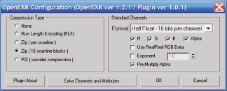
10.  Change the file type to OpenEXR, give the sequence of images a name, and click the Save button. The OpenEXR Configuration dialog box appears.

11.  Change the Format type to Half Float – 16 bits per channel and leave all other settings as is. We are using the OpenEXR image format because of its many advantages, such as a high-dynamic range pixel format, good compression, numerous sub-channels, and more.

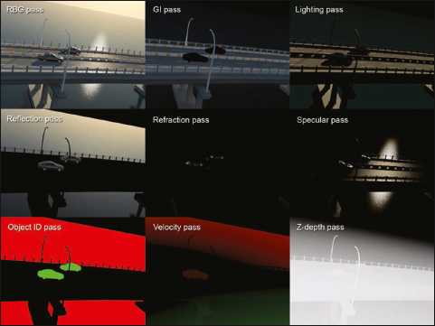
12.  Go to the Render Elements tab. Here you can see we have numerous render elements listed. These represent all the different channels of information that will be rendered out as separate EXR files to the location you just specified. These channels include things such as motion blur, depth-of-field, global illumination, and many others. Later we’ll explore these channels in greater depth when they’re used in Fusion. Although they are presently listed here, they are not yet activated.

13.  Enable the Elements Active option.

14.  Render the animation, or just a portion of it if you only want to render a small test sequence. Rendering all 250 frames of this animation will take approximately 12-24 hours, or 3-6 minutes per frame, depending on your computer’s speed. The next illustration is an example of what the various render elements of frame 150 should look like. To see what the compiled raw animation looks like at this point now, play the movie bridge_01_day_raw.mov.

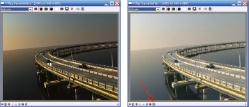
At the bottom of the V-Ray frame buffer (i.e., V-Ray version of the rendered window) is a button labeled sRGB. This button changes an image’s gamma from 1.0 to 2.2. The next illustration shows what both versions look like, and later we will explore the difference between these 2 values.

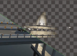
The final step of the rendering process is to calculate an ambient occlusion pass to bring more realism to our animation. Ambient occlusion (AO) is the measure of how much of the sky is occluded, or blocked from view, at any given point on a surface. An AO image is always grayscale, and an example is shown in the following illustration. As you will see shortly, creating an AO pass will do wonders for our final animation because it will be used within Fusion to multiply the colors of the animation, which will add depth and contrast and create a weathered look to surfaces that would otherwise look too perfectly clean.

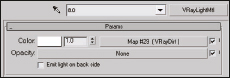
To make an AO pass in V-Ray, we need to apply a special material to all of the objects in the scene. Specifically, we need to create a VRayLightMtl, which is a material that casts illumination. The strength and color of the illumination is dictated by the color or color channel shown in the following illustration. By loading a special map type, the VRayDirt map, we can use the map to control the strength of the VRayLightMtl. The VRayDirt map wants to generate a grayscale image where pure black areas represent completely occluded points blocked from view of the sky, and pure white areas represent completely unoccluded points. In between pure black and pure white are areas that are partially occluded. By using this map in the Color channel of the VRayLightMtl, we can create a nice AO pass, like the one shown in the previous illustration. Incidentally, it should be no surprise that an AO pass is also known as a dirt pass since its greatest benefit is the way it creates a weathered look to objects in a scene.

15. Open scene ch16-03.max. In this scene, the following changes were made to prepare an AO pass for render:

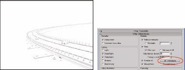
•   A new VRayLightMtl was created and the VRayDirt map was added to the Color channel, as shown in the previous image. Within the VRayDirt map, two settings were changed from their default value. First, a Radius value of 0.3m was used instead of 10m, to make the occlusion not spread out so far, as shown in the left image of the following illustration. Second, a subdivs value of 16 was used instead of 8. This helps reduce noise in the rendering.

•   An instance of this new VRayLightMtl was dragged into the Override mtl channel as shown in the right image of the following illustration.

•   Indirect Illumination was turned off because it’s not needed in the calculation of an AO pass.

•  Render Elements were turned off in the Render Elements tab.

•   In the Global switches rollout, the Shadows and Lights options were disabled, as shown in the right image of the following illustration, because we don’t want these lights or shadows affecting the AO rendering.

•  In the Environment and Effects dialog box, the VRaySky map used as the background was removed and the background color was changed to pure white.

•   In the Frame buffer rollout, the saved file name was changed.

•   Render the AO version of the animation. This type of rendering should take very little time to render because it doesn’t use GI, textures, reflections, etc. The left image of the following illustration shows what frame 0 should look like. Notice the difference between this image and the previous AO image. The difference in the two images is a result of using a smaller radius value.

The Compositing Phase

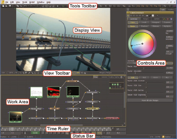
Before we start an exercise on compositing with Fusion, a brief overview of its interface is in order. Fusion can be divided into the following main areas:

•   Tools Toolbar – This displays shortcuts to some of the critical tools available in Fusion.

•   View Toolbar – This displays additional commands for polylines, text, and motion paths.

•   Display View – The Display View is used to view the images produced by tools in the flow. The view can be configured as a single view or two separate views located side by side, using the layout buttons in the view toolbar. Additional floating views can be created on demand from the view menu.

•   Work Area – The Work Area displays the Flow, Console, Comments Tab and Timeline and Spline Editors. For more information, see the chapters on Flow Editor, Timeline Editor, and Spline Editor.

•   Controls Area – The Controls Area displays controls for the tools in the flow. Additional tabs in this area reveal controls for any masks or modifiers attached to the currently selected tool.

•   Time Ruler – The Time Ruler displays controls global to the project, such as the current frame, render range, proxy and quality modes, and so forth. Buttons for playing, navigating, and rendering the flow are also located here.

•   Status Bar – The Status Bar displays various bits of information about whatever is beneath the mouse pointer, the time to render completion and render status, and memory in use.

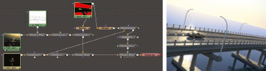
1.  Start Fusion with a new composition. Composition is the word used to describe a working Fusion file, and appropriately enough, the files are saved with the extension .comp.

2.  Within the Tools Toolbar, click the LD icon. This activates the Loader tool, which automatically opens a window in which a sequence of image files can be selected. Instead of listing every individual file within a folder, Fusion will display a sequence of files with a single name and a suffix showing the sequence range involved.

3.  Select the sequence 1.RGB_color.0125-0150.exr and click Open to load this sequence of images. For simplicity, we will only use 1 second of the animation; however, you can render the entire sequence as previously described if you desire.

The only thing you see at this point is a single icon in the Work Area, as shown in the left image of the following illustration. If you put your cursor over the icon, a flyout appears containing two black dots. These dots represent the two display views above the Work Area.

4.  Click the black dot on the left, as shown in the right image. This causes the sequence of images to be displayed in the left window of the Display View. We don’t need two windows open at the same time so let’s make it a single view.

5.  In the Tools Toolbar, click the icon representing a single display view, as shown in the following illustration. The two display views should change to a single display view.

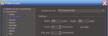
6.  From the File menu (above the Tools Toolbar), select Preferences and then click on Frame Format, as shown in the following illustration.

7.  Click on the Default Format drop-down list and select NTSC (Square Pixel), and within the Settings section, enter a Frame value of 25. This change causes the default frame resolution to be 640x480 and the frames per second rate to be 25. Click the Save button to complete the configuration.

At the bottom of the Work Area is the Time Ruler, where we should set the frame count to match the sequence of images loaded. There is a quick and easy way to do this.

8.  Click and drag the loader icon from the Work Area to the Time Ruler. Release the mouse and the Time Ruler should change to reflect the total number of frames you loaded a moment ago. Some versions of the software may require you to simultaneously hold the Shift key while you drag the loader.

The image loader in the Display View looks like the original image before we used the option in the VRay frame buffer to display the image with a gamma value of 2.2. Let’s do the same thing here that was done in the VRay frame buffer. As mentioned before, we are going to use linear color space for compositing, and a little later we’ll see why.

9.  Within the View Toolbar, click the LUT icon, as shown in the following illustration, and then click Edit. The LUT Editor appears.

10.  Set the Color Gamma to 2.2 and close the window. The image shown in the Display View changes to reflect a gamma value of 2.2. This is the same change made within the VRay frame buffer using the sRGB icon.

11.  Within the Time Ruler, click the Play icon to play the sequence of images.

12.  Save this composition. If you want to continue on from this point with an already saved file, load the composition ch16-01.comp.

The first composite we will make is to add the ambient occlusion pass to the sequence.

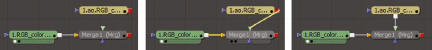
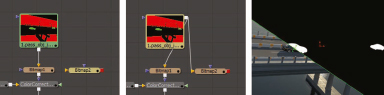
13. Click on the 1^st icon you created in the Work Area. If you do not have this icon selected, it is displayed as a green icon. If you do select it, it’s displayed as a tan icon and its name (Loader1) is displayed in the Controls Area, where you can do things like change the files used and change the number of frames loaded.

With the Loader1 selected, as shown in the left image of the following illustration, click the LD icon in the Tools Toolbar. Select the sequence 1.ao.RGB_color.0125.exr and click Open to load the sequence. Notice that when you created this new loader, two new icons appear in the Work Area. One is the new loader icon and the other is a merge icon. This icon represents the Merge Tool. Had you not had the Loader1 icon selected when you clicked on the LD icon, this merge icon would not have been created. But since you did have it selected, Fusion assumes that you want to merge the two loader sequences together. You could have clicked on the Mrg icon instead, followed by the LD icon, and could have then created the linking you see in the right image manually. It is critical to know how to do this, so instead of continuing on from here, let’s revert back to a moment ago.

14.  Undo the Add Loader command you just executed. The Work Area returns to displaying Loader1 only.

15.  Click and drag on the Mrg icon in the Tools Toolbar and place it directly to the right of Loader 1 in the Work Area, as shown in the left image of the following illustration.

16.  Place your cursor over the red square on Loader1. Notice that in the Status Bar, it says that this is Loader1 Output.

17.  Place your cursor over the yellow arrow of Merge1. Notice that in the Status Bar, it says that this is Merge1 Background.

18.  Click and drag from the Loader1 Output to the Merge1 Background and release the mouse. When you do, a link is drawn between the two icons. You have just told Fusion to load the sequence of images in Loader1 as the background of Merge1.

19.  Click and drag on the LD icon in the Tools Toolbar and place it directly above the Merge1 icon in the Work Area, as shown in the left image of the following illustration.

20.  Click and drag from the red square of Loader2 to the green arrow of Merge1, as shown in the middle image. When you do, a link is drawn between the two icons, and Fusion changes the positioning of the square to the bottom of the loader (right image). By doing this, you have just told Fusion to set the ambient occlusion sequence as the foreground of the merge tool.

At this point, we should view the composite we just created. We can split the current window into 2 windows, so we can compare a before and after view side-by-side.

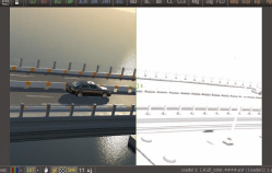
21.  Click the Switch to A/B split view icon in the View Toolbar, as shown in the following illustration. The image that is loaded is split vertically and we can only see the left side in channel A.

22.  Carefully click and drag the Loader2 icon (AO pass) from the Work Area to the right side of the vertical green line in the Display View. When you do, the AO pass is loaded in channel B. You could press the play button now to play both sequences of images.

23.  Click the LUD icon in the View Toolbar, select Edit, and change the Gamma Color from 1.0 to 2.2.

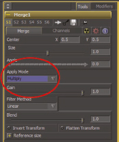
24.  Drag the Merge1 icon from the Work Area to channel B of the Display View. When you do, nothing changes. The reason nothing changes is because we have set Loader1 as the background of Merge1 and Loader2 as the foreground. Since the foreground covers and hides the background, we don’t see the original rendered sequence. The whole purpose of creating the AO pass was to use it to multiply the colors of the original animation, not to hide the original animation.

25.  Click on Merge1 and within the Control Area, click on the Apply Mode drop-down list, shown in the following illustration, and then select Multiply. This causes channel B to show the effect of multipling the original animation color by the AO pass. You can consider pure white to represent a value of 1 and pure black to represent a value of 0. So in all of the pure white areas of the AO pass, the original animation is unaffected. In areas of the AO sequence where you see gray, the result will be a reduction in color value, with greater reductions being applied to darker AO areas.

26.  Click and hold on the green vertical line and drag around the Display View. Notice that you can rotate the green line, as shown in the following illustration. Notice also that there is a square in the center of the green line. You can move the entire line by dragging from this square.

27.  Position the green line as shown in the right image of the following illustration. When you do, you can see quite clearly the effect of the AO pass on the white concrete barriers. Without the AO, the concrete looks too flat and clean. By adding the AO, we add a layer of dirt, which adds depth and realism to the animation.

28.  Save your composition. If you want to continue from this point on, open the file ch16-02.comp.

Up to now, the three icons we have been working with in the Work Area have been displayed without the benefit of any visual aid in what they represent. We can change that.

29.  Right-click over any empty part of the Work Area, and from the menu that appears, select the Force Source Tile Pictures. The Work Area icons change to display a thumbnail view of the various sequences, as shown in the right image of the following illustration. You may have to reposition the thumbnails slightly if they are positioned too close to each other.

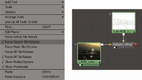
30.  Right-click over any empty part of the Work Area, and from the menu that appears, select the Force Source Tile Pictures. The Work Area icons change to display a thumbnail view of the various sequences, as shown in the right image of the following illustration.

Now it’s a time to make some color correction of our image and explore masks.

31.  Click the Merge1 icon. It should turn tan.

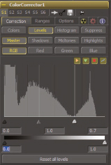
32.  With the Merge1 icon selected, click on the CC icon in the Tools Toolbar. Rather than placing the CC icon yourself and having to manually link it to the Merge1 icon, selecting the Merge1 icon before creating the CC icon makes the process a little easier. Color correction is a powerful tool that let’s you change gamma, brightness, contrast, saturation, levels, and much more. Let’s start by making an adjustment to the levels in the animation.

33.  From the Controls Area, click the Levels button and enter a value of 0.7 in the field shown in the following illustration. This should increase the contrast of our animation, but in the Display View nothing has changed. The reason why is because we have not yet loaded ColorCorrector1 into either channel A or B.

34.  Drag and drop the ColorCorrector1 icon from the Work Area into channel B of the Display View. When you do, the total combined result of everything coming into ColorCorrector1 and the result of ColorCorrector1 itself should be displayed in channel B.

Now let’s really make some ingenious adjustments.

35.  Select ColorCorrector1 and click the CC icon again in the Tools Toolbar. A second color correction icon is loaded and connected to the first.

36.  With ColorCorrector2 selected, click the Bmp icon in the Tools Toolbar. This is the BitmapMask Mask tool and once loaded, it is automatically linked to feed into ColorCorrector2.

Rather than using the method we’ve been using, where we select an icon in the Work Area and then click on an icon in the Tools Toolbar, we will have to manually link the next tool.

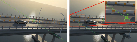
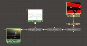
37.  Click and drag a new loader icon from the Tools Toolbar into the Work Area directly above the Bitmap1 icon. When the explorer window opens, select 1.pass_obj_id.0125-0150.exr. This is the rendering element we created by establishing different material IDs for the various objects. In this scene, we set the water object to material ID 1 and the car object to material ID 2 (green color).

38.  Click and drag this new loader icon (Loader3) into channel B of the Display Area.

39.  Click and drag from the red square of Loader3 (Output) to the yellow arrow of Bitmap1 (Background). The result of the flow thus far should look like the following image. The work flow is often used because this sequence of inputs and outputs is basically a flowchart of information.

40.  Load ColorCorrector2 into channel B of the Display View.

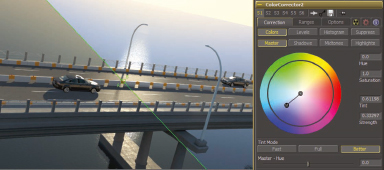
41.  Select ColorCorrector2 in the Work Area and then select the Colors button in the Controls Area (if not already selected).

42.  Click and drag from the center of the color wheel out and to the right until channel B changes to a red hue as shown in the following illustration.

The intent in creating a material pass and loading it into the flow is so we could use it to apply color correction to very precise areas of the animation. Let’s make the color correction change we just made apply only to the water in the scene. The water was given a red material ID, so we can use this to isolate the effect of the color correction.

43.  Select the Bitmap1 icon and in the Controls Area, select Red from the Channel drop-down list, as shown in the following illustration.

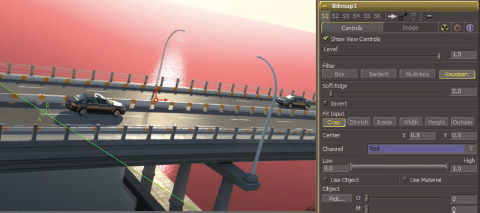
44.  Drag and drop Bitmap1 to channel B view to see the mask. You’ll see a black and white image, where only the white area is allowed to be affected by the color correction applied.

45.  Drag and drop ColorCorrector2 to channel B again so we can fix the color of the water.

46.  Select ColorCorrector2 in the Work Area and within the Color tab of the Controls Area, change the color of the water so it’s a fairly rich blue color, as shown in the following illustration. Be careful not to add so much Strength that the water is unrealistic. Notice that the Strength value changes as you drag around within the color wheel.

47.  Save your composition. If you want to continue from this point on, open the file ch16-03.comp.

Now let’s add some glows and highlights to the animation.

48.  With ColorCorrector2 selected, click on the LD icon once again in the Tools Toolbar. Merge2 is automatically generated with CorrectCorrect2 linked to the background and the new loader linked to its foreground.

49.  Select the 1.pass_specular.0125-0150.exr sequence. This is represents the specular highlights channel. As before, it’s helpful to select the icon you want the new loader to link to, because the new loader is automatically placed in a suitable location in the Work Area and aligined in an aesthetically pleasing fashion. This can be seen in the left image of the following illustration.

50.  Drag and drop the new loader (Loader4) into channel B of the Display Area.

51.  Select Loader4 and from the Tools menu select Matte > Luma Keyer. The Luma Keyer Tool uses the black and white specular channel to create an alpha channel. This alpha channel can then be used as a mask for other effects so we can adjust the specular highlights without affecting any other part of the image.

52.  Drag Lumakeyer1 to channel B of the Display View to see what this layer of information looks like, and within the Controls Area turn off the Post multiply image option. In the following illustration, we can see only bright pixels.

53.  Drag and drop the Merge2 icon into channel B to see the combined effect of all flow elements at this point.

54.  Select LumaKeyer1 and from the Tools menu, select Blur > Soft Glow. Notice that a glow is applied to only the areas that were already bright in the scene, as determined by the specular channel we just added.

55.  Within the Controls Area, change the Blend amount to 0.5.

Now let’s make some highlights on the cars. To do this, we need to isolate the cars’ specular channel from other objects.

56.  Drag and drop a new BitmapMask Mask icon directly to the right of Bitmap1, as shown in the left image of the following illustration.

57.  Connect the Output of Loader3 to the Input (background) of Bitmpa2, as shown in the middle image.

58.  Drag and drop Bitmap2 into channel B of the Display Area. All you should see is solid white because Bitmap2 is set to display its alpha channel by default. Since Bitmap2 is fed by Loader3, which has no alpha channel, white is the only thing it can display.

59.  In the Controls Area, change the Channel to Green. When you do, you should see the cars in white and everything else in black, as shown in the right image of the following illustration.

60.  Within the Controls Area just above the Channel setting, enable the Invert option.

Since we want to adjust the specular highlights on just the cars, we need to create an alpha channel of just the cars’ specular highlights. To do this, we need to combine the alpha channel of the entire scene’s specular highlights (LumaKeyer1) with the alpha channel of the cars (Bitmap2). This is what the Matte Control tool allows us to do.

61.  With Bitmap2 selected, click on the Mat icon in the Tools Toolbar. This loads the Matte Control tool.

62.  Create a link from the LumaKeyer Output to the MatteControl1 Input, as shown in the left image of the following illustration.

63.  Drag MatteControl1 to channel B of the Display View. The result is just an alpha channel created from the specular highlights (right image), which is all the work of LumaKeyer1. This is not what we want. We want to create an alpha channel of just the cars’ specular highlights. By default, when we created MatteControl1, the link from Bitmap2 was to the wrong place.

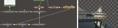
64.  Click and drag the blue arrow leaving Bitmap2 and place it on the white arrow of MatteControl1, as shown in the left image of the following illustration. The white arrow is called the Garbage Matte. As its name implies, the Garbage Matte allows you to throw away that part of LumaKeyer1 that is not part of Bitmap2. The result is an alpha channel of just the cars’ specular highlights, as shown in the right image.

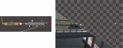
65.  Select MatteControl1 and from the Tools menu, select Effect > Highlight, and reposition the new highlight tool directly below MatteControl1, as shown in the left image of the following illustration.

66.  Drag Highlight1 to channel B.

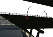
67.  In the Controls Area, change the Low value to 0.75, change the Length value to 0.65, and change the Number of points value to 6. The result is a nice streak to the cars’ highlights, as shown in the right image.

Now let’s add color to the highlights.

68.  With Highlight1 selected, add a color correction tool and reposition it just below the Highlight1, as shown in the left image of the following illustration.

69.  Drag ColorCorrector3 to channel B.

70.  Adjust the color of the cars’ specular highlights using the color wheel in the Tools Area, as shown in the following illustration.

Now we need to show the result of all the work performed thus far.

71.  Drag and drop a new merge tool from the Tools Toolbar and place it below ColorCorrector3, as shown in the left image of the following illustration.

72.  Create a link from the Output of Merge2 to the background of Merge3.

73.  Drag Merge3 to channel B.

74.  Create a link from the Output of ColorCorrector3 to the foreground of Merge3, as shown in the right image.

At this point we are finished with this portion of the composite process and we need to save the output. You can also play the final sequence of images to see the result.

75.  Select Merge3 and click the SV icon in the Tools Toolbar and select a file type and save location. You can save your file type as JPG to keep file sizes down with no negligible loss in quality.

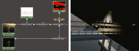
76.  Click the green Render button to start the process of creating each individually composited frame. The finished result should look similar to the following illustration. If you want to explore the final composition file, open ch16-04.comp.

Summary

The goal of this chapter was to introduce you to the power and utility of compositing with professional 3^rd party software. We hope you agree that compositing with great software like Fusion is really quite simple in comparison to a program like 3ds Max. Although it is beneficial to create your 3ds Max scenes as complete and finished products, there is no denying the usefulness of software that can do some of the things this chapter illustrated. Like other chapters in this book, we have only brushed the surface of what is possible. As we alluded to earlier, we can make adjustments to objects based on their distance from the camera, their speed, or any number of things that could fill a book by itself. The tools are in the program to do more things than you can probably imagine.