
CHAPTER 10
Creating Vegetation
UNLIKE THE CREATION OF MOST object types in visualization, creating vegetation is more an art than a science. When you create walls, roofs, sites, and most other scene elements, you usually do so with the precise guidance of architectural or engineering drawings. Even though we reserve a certain degree of artistic interpretation in the creation of many object types, especially in the absence of information, that degree usually extends much farther with vegetation. For example, when a set of architectural drawings specifies that the roof of a house needs to be a barrel tile roof, it probably doesn’t matter if the roof is barrel tile or Spanish tile, but it certainly needs to be some kind of tile, rather than a completely different roofing material such as standing seam or asphalt shingles. On the other hand, when a landscape drawing specifies the placement of an oak tree, you can often substitute a completely different tree, such as an elm. When you place the front door of a house, that door needs to be placed with precision. On the other hand, the location of a tree is often guided less by a landscape drawing and more by where it can block the view of something you don’t want the camera to see. These are just a few examples of the added latitude that we are usually afforded in the creation of vegetation as compared to the creation of most other object types. Furthermore, landscape drawings are often never provided, in which case we are sometimes asked to play the role of landscape architect.
Because of the artistic nature of creating vegetation and the myriad issues that challenge our computers’ resources, vegetation is one of the most difficult elements of a 3D scene to simulate realistically. This is especially true when your scenes are animated, and your cameras move in and around the vegetation. Whether a scene contains 2D vegetation, 3D vegetation, or a combination of both depends on numerous factors, such as rendering time available, your vegetation libraries, distance of the vegetation from the camera, camera paths, and available RAM. Improperly created vegetation can lead to extremely large file sizes, excessive rendering times, or even system crashes.
So how do you add thousands of trees and plants to your scenes without crashing 3ds Max or without taking weeks to render? Furthermore, how do you even place the vegetation without taking endless hours to do so? The solution can be elusive and is completely scene dependent, but the following is a discussion on some considerations that may make the solution easier to find.
Types of Vegetation
Vegetation in a visualization can be categorized in one of two ways; 2D or 3D. 2D vegetation is represented by imagery and 3D vegetation is represented by a large number of small polygons that together simulate the physical structure of a certain type of vegetation. For each type, there are several methods of implementation and endless tips and tricks to be used. But before jumping into a discussion about effective methods of creation and placement, let’s look closely at both vegetation types and the pro and cons of using each.
3D Vegetation
It wasn’t many years ago when the idea of using 3D vegetation in a scene was considered ridiculous and impractical. When the 1st version of 3ds Max came out, most top visualization firms relied heavily, if not completely, on 2D vegetation. The few firms that did implement 3D vegetation were usually only able to place just a few examples very close to the camera, and most of those were hand crafted and still relatively low polygon compared to today’s standard. Today, 3D vegetation is the standard.
Sometimes containing hundreds of thousands of polygons per example, 3D vegetation, like the one shown on the left side of Figure 10-1, provides an undeniable degree of realism over 2D vegetation, like the one shown on the right. Sometimes that realism isn’t always needed or justified, such as trees off in the distance, but when it is needed, using 3D vegetation can truly make or break a scene.

Figure 10-1. An example of a 3D vegetation (left) and 2D version (right).
The obvious advantage of 3D vegetation is that it looks 3D. It has depth and looks different at every angle. Not only does it cast great shadows, unlike 2D vegetation it also casts realistic shadows on itself, which is a tremendous advantage that adds to its depth. Another tremendous advantage is that you can view the vegetation from any angle, unlike 2D vegetation, which can look distorted when viewed at high angles and strange when not viewed from the same angle from which the image was captured.
The obvious disadvantage with this type of vegetation is that it significantly increases your refresh rate and render time. 3D vegetation slows render times because of the faces that must be rendered and because of the shadows that must be accounted for.
Unfortunately, 3ds Max presents an extremely meager, and for all practicality, useless selection of 3D vegetation. Fortunately, there are numerous 3D software packages available today that can satisfy your needs in this area.
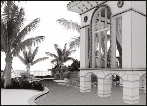
When we first started implementing 3D vegetation in our scenes at 3DAS, like most firms we were forced to create vegetation from scratch, sometimes spending an entire day to create one tree or plant. Over the years we spent many hundreds of man-hours building our own custom vegetation library, only to abandon most of it for the more realistic vegetation we can produce in a fraction of the time with a software package called OnyxGarden Suite for Onyx computing (www.onyxtree.com). This is a series of plant generator programs that run outside 3ds Max and work in conjunction with a plug-in that runs within 3ds Max. The software is relatively easy to learn and we highly recommend its use for anyone in the 3D visualization industry regardless of skill level. It provides great functionality for creating just about any type of vegetation you can imagine and when combined with good materials and lighting, the results are simply amazing. You can even step up the quality of your animations by having the vegetation blow in the wind. All of the vegetation shown in Figure 10-2 was created using Onyx software.
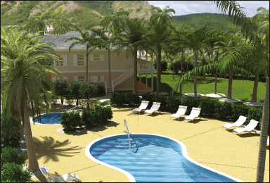
Figure 10-2. 3D vegetation created entirely with software from Onyx Computing.
Virtually all of the 3D vegetation used in our work is created with Onyx, but regardless of which software you choose, you will have to use 3rd party software of some type to create your own 3D vegetation in a reasonable amount of time.
2D Vegetation
There is only one reason I can imagine for which anyone would not want to use highly detailed, well-crafted vegetation models; to reduce the consumption of system resources and to reduce render times. But until computers are able to render in real-time, users will always be looking for ways to do just this. Needless to say, there will probably be a place for 2D vegetation for many years to come, and because of this, part of this chapter is dedicated to implementation of 2D vegetation in a useful and worthwhile manner.
Mesh and Poly Based 2D Vegetation
There are two main types of 2D vegetation; imagery represented by Edit Mesh or Edit Poly objects or imagery created through the use of a plug-in. With the first type, vegetation is usually represented by an image placed on two criss-crossed polygons, and an image in the opacity channel to mask areas of the object where the vegetation does not show. When the left image in Figure 10-3 is placed in the diffuse channel of a material, and the middle image is placed in the opacity channel, you are able to simulate the appearance of 3D vegetation, as shown in the image on the right.

Figure 10-3. Using opacity maps to create 2D vegetation.
The greatest advantage of the criss-cross vegetation type is that it requires only four faces (or two polygons) per object, and therefore it renders quickly. This makes rendering a forest of trees very easy, and although they might not be suitable for close-up views, the ability to populate your terrain stretching to the horizon is invaluable.
Another advantage of this criss-cross vegetation type is that all objects with the same vegetation material can be attached together as a single object. When creating a large amount of vegetation, the importance of this advantage cannot be overstated. As we’ll discuss later in this chapter, the number of objects in a scene is a critical factor in the time it takes to render. All of the trees in Figure 10-4 are part of the same object (not to be confused with being part of the same group). Still another advantage is that you can populate your scene extremely fast with this type of vegetation. When done correctly, you can create thousands of trees and all the shrubs and flowers your scene needs in just minutes, regardless of the size of your scene.
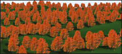
Figure 10-4. A forest of 2D trees placed with a few clicks of the mouse.
The greatest disadvantage of using criss-cross vegetation is that the images become distorted when viewed at high perspectives, such as those greater than 45 degrees above the horizon, as shown in Figure 10-5. This makes camera placement critical and accentuates the need for determining placement as early as possible. One of the production tips at the end of the book discusses the need to create an animation script as early as possible. For an animation where cameras move in and around a scene, knowing exactly where a camera will go and where it will see will help you better decide where to place high polygon 3D vegetation and where you can get away with using 2D vegetation.

Figure 10-5. The negative effect of distortion for 2D trees viewed from high angles.
Another disadvantage of this type of object is that it often casts poor shadows. Most shadow types, such as raytracing and advanced ray-tracing, allow you to take advantage of the image in the opacity channel and cast shadows that mimic the shape of the vegetation. Ray-traced shadows are automatically configured to trace opacity maps, while advanced ray-traced shadows require you to enable the Transparent Shadows option in the Optimization rollout. However, shadows cast through the tracing of opacity maps do not always look good, regardless of the shadow type or render engine used. This is especially true when the sun in a scene is placed very high or very low in the sky, but even when placed at the best possible angle (i.e., 45 degrees up in the sky), these shadows usually appear stretched and distorted. This is not to say that you cannot or should not use this type of shadow. It is in fact a very good option for scenes where the sun is not placed too high or too low, as shown in the right image of Figure 10-6, and it is especially good for 3D terrain where some of the other tricks described later in this chapter won’t work. When used with 3D terrain, the shadows fall on surrounding objects and conform to the slope of the surrounding terrain, unlike some of the faked shadows that only work well with 2D terrain and without other objects around.
As an additional note, I don’t recommend use of the shadow map type for the sun in a scene. Shadow maps, which are already very memory consuming, do not allow the tracing of opacity maps and instead cast shadows of the entire object, as shown in the left image of Figure 10-6.
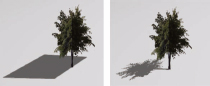
Figure 10-6. 2D shadows with and without the tracing of opacity maps.
Yet another disadvantage of using 2D vegetation is their tendency to be illuminated very poorly. Without handling this type of vegetation properly, it is usually easy to see one half of the tree illuminated completely different from the other half. Shortly, we’ll look at ways to alleviate this particular problem as well as ways to create far better shadows for 2D vegetation. Furthermore, we’ll see how to do these things in ways that don’t require you or your computer to work too hard.
Plug-in Based 2D Vegetation
Another type of 2D vegetation can be created with a plug-in that uses a dummy object to set the position, rotation, and scale of the object. The most widely used example of this is the RPC (Rich Photorealistic Content) plug-in, shown in Figure 10-7. This type of vegetation looks much better than mesh and poly-based vegetation because a different image is generated from different perspectives and because you always see a full image straight-on. Another advantage is that when used in moderation, they render much quicker than 3D vegetation, although not as quickly as the criss-cross vegetation.
Unfortunately, the disadvantages of this type of vegetation are numerous. RPCs are memory hungry because all of the individual images that represent the vegetation from each unique perspective must be loaded into RAM at the start of the rendering process. When too many are used, they can swallow up all of the available RAM in your computer and leave you with nothing left to render. Another disadvantage is that they cannot be attached together, and therefore must remain as individual objects. The result can be much greater rendering times. Still another disadvantage is that they cannot be placed as quickly as the criss-cross vegetation type because they cannot take advantage of some of the great placement tools 3ds Max has to offer, such as the Scatter command.

Figure 10-7. An example of an RPC (Rich Photorealistic Content).
Creating 2D Vegetation
In the first few years we worked on visualizations at 3DAS, no other element in a scene caused more frustration and late nights than vegetation. We tried just about every conceivable approach to creating realistic looking trees, shrubs, and flowers in an efficient and cost-effective manner. Some worked well and some did not. Some methods that used to be great with previous versions of 3ds Max and 3d Studio for DOS have been made obsolete by new program features or new plug-ins. But nevertheless, until computers reach real-time speed regardless of the quality of the rendered output, there will always be a few fundamental procedures that can save you countless hours in the course of a visualization project. In this next section, we will look at some of these procedures.
Creating 2D Trees
When you do decide to use 2D trees, perhaps the most efficient way to create it on a large scale is by using the Scatter command. The Scatter command is used to create copies of one object over the surface or within the volume of another object. In this way, it gives you a quick and easy method to create realistic vegetation for an entire project, regardless of size. Creating vegetation this way can produce effective and realistic results with minimal burden on your computer. As mentioned earlier, it’s often unimportant to the clients exactly what type of trees and plants they see in their visualization and since landscape drawings are usually one of the last things created during a project’s planning, landscaping will often not even be decided by the time your work begins. When this is the case the client may want you to play landscaper and tell you to simply create something that looks good. This can be a double-edged sword. Although it is nice to not be constrained by placing the exact required vegetation type throughout your scenes, the client may not like what you use. Good communication about landscaping requirements and exactly how you will meet them cannot be overstated. In fact, if anything should be highlighted in your contract, it should be details regarding the landscaping. Whenever possible, we highly recommend gaining flexibility from the client in this area.
When you aren’t constrained by creating vegetation of a particular type, I recommend using the Scatter command to create at least a portion of your plants. Doing so can save an enormous amount of time, especially for larger projects. Some projects call for the use of thousands of trees and plants, and placing each of these any other way can take many hours. With the Scatter command, you can create the appearance of a beautifully landscaped scene in a fraction of the time.
Scatter - The ‘Area’ option
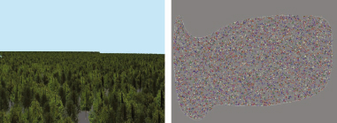
The following 2 exercises illustrate 2 different methods of using the Scatter command to efficiently place a large number of 2D trees in a very short amount of time. In this 1st exercise, we will place the 2D trees shown throughout the background of the images in Figure 10-8. This exercise will not involve the illumination of these nor will it involve the creation of shadows. Both of these will be discussed later in the chapter.
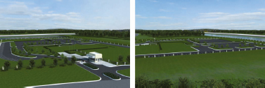
Figure 10-8. A scene with thousands of 2D trees.
Creating 2D Trees – Method #1 (Scatter with the Area option)
1. Open the file ch10-01.max. This scene contains six 2D criss-cross trees, an editable spline that represents where the trees will be scattered, and a camera. Incidentally, there are 2 versions of each tree type. Whenever using 2D vegetation, it’s helpful to use more than one version of each vegetation type so a repetitive pattern isn’t obvious.
2. Select the object Tree-Area and add the Edit Mesh or Edit Poly modifier.
3. Select the object Site-2D-Tree-Ash-A.
4. Select Create > Geometry > Compound Objects > Scatter.
5. Click the Pick Distribution Object button and click on the object Tree-Area.
6. Open the Display rollout and enable the Hide Distribution Object option.
7. In the Scatter Objects rollout, change the Duplicates value to 5,000.
8. In the Distribute Using section, enable the Area option. This provides the best distribution spacing for vegetation.
9. Open the Transforms rollout and type a value of 90 for just the Rotation Z field. This randomly rotates each face +/- 90 degrees about each tree’s Z axis.
10. Render the Camera view. Notice that the trees appear to have a white haze around their outer edges. This is because of the white color applied to the Diffuse and Ambient color channels. 2D criss-cross vegetation should always have a pure black color applied to these channels even when maps are used. The antialiasing applied to the edge of the cutout image picks up and borrows from these colors, so they always need to be set to pure black. As a good rule of thumb, the Specular color should also always be set to pure black because if specular highlights are present the vegetation would show these highlights in the masked area of the image.
11. Open the Material Editor.
12. Select the material Site-2D-Tree-Ash-A and change the Diffuse and Ambient and Specular colors to pure black and render the Camera view again. The white haze is removed. Notice also that some trees appear to be very narrow. This is because the tree material is single-sided and some are seen at an angle nearly parallel to the camera’s view.
13. Enable the 2-Sided option for the material Site-2D-Tree-Ash-A. This essentially doubles the number of visible trees, although some render engines (such as V-Ray) generate 2-sided materials automatically.
14. Add the Edit Mesh or Edit Poly modifier to the object. Notice that the trees are now visible in the Camera viewport.
15. In the root of the Site-2D-Tree-Ash-A material, enable the Show Map in Viewport option. The trees are now shown as cutouts from their background. This option has to be enabled in the root of the material rather than within the Diffuse Color channel or it will not cut out the background of the tree image.
16. Repeat the previous steps by scattering all 5 trees, each time using a unique Seed value so the trees are not scattered in the exact same position.
17. Render the Camera view again. The result should look similar to the left image of the next illustration. The right image shows a close-up top view of one area. Rendering 30,000 trees like this should only take a few seconds. If you want to see a completed version of this exercise, open the file Ch10-02.max.
Scatter – The ‘All Face Centers’ option
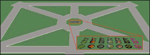
If you’re fortunate enough to have landscape drawings at the time you need to create the vegetation for your project, which seems to be less than half the time for our firm, you might want to take advantage of the CAD linework already in place. Using this method, you replace the landscape symbols inside AutoCAD with a simple triangle, import the triangles into 3ds Max, apply the Edit Mesh or Edit Poly modifier, and use the Scatter command to place a tree at the center of each face (i.e., the triangles you imported).
If you’re even luckier to have landscape symbols as blocks, this routine is even more effective. When the symbols are blocks, all you have to do to create the triangles globally inside AutoCAD is replace the linework in a block with a triangle. By resaving the block with new linework, you can change every instance of that block automatically. Once this is done, simply explode all of the blocks and import the linework into AutoCAD by layer.
Figure 10-9 shows an example of this method. The left image shows an AutoCAD drawing with the triangles that were created and the right image shows an aerial view of the finished project including the landscaping that was scattered on these imported triangles. The landscape in this particular project was almost completely 3D because of the need to see aerials like this. This process, however, is identical regardless of whether you use 2D or 3D vegetation. The entire process was very quick and took only a couple of hours. While creating decent 3D vegetation for this scene could actually be accomplished in just a few minutes using other techniques described later in this chapter, the benefit of this particular method is that you can place the precise vegetation called for in their exact locations, which is sometimes very necessary.

Figure 10-9. An example of scattering vegetation using the All Face Centers option.
Creating 2D Vegetation – Method #2 (Scatter with the All Face Centers option)
The following exercise describes the process for using the Scatter command with the All Face Centers option. AutoCAD is required to use the process described; however, the following is simply a description of the process and does not require the opening of any files.
1. Open the AutoCAD landscaping drawing in which you want to create vegetation.
2. Choose a landscape block you want to turn into a triangle and double-click on the block or select the block and type RefEdit.
3. Create a new layer and give it the name of the tree you want to scatter.
4. Make the layer you created the current layer.
5. Create a 3-sided closed pline (not spline) in the center of the block.
6. Delete the existing linework that makes up the block you are editing.
7. Type RefClose to save and close the block editing feature. All the blocks with the same name will now appear as triangles.
8. Repeat steps 1 through 5 for all landscaping blocks.
9. Explode all of the landscape blocks.
10. Import the linework into 3ds Max using the option to make all linework on the same layer be part of the same object.
11. Add the Edit Mesh of Edit Poly modifier to the imported triangles.
12. Use the Scatter command as you did in the previous exercise, except this time, use only one duplicate and instead of using the Area method for distribution, use the All Face Centers option.
Illuminating 2D Trees
Perhaps the biggest drawback users find in creating 2D criss-cross vegetation is the poor illumination that usually plagues its use. The reason for this is because the light in the scene does not evenly illuminate the 2 polygons that make up the tree. To ensure that the illumination is even, you must first ensure that the 2D vegetation does not cast shadows on itself (or on anything else), and that enough lights are used to cast equal illumination in all directions around the perimeter of all trees. The first part of this is simple - just turn off the Cast Shadows and Receive Shadows option for the trees (in the Properties dialog box of each object). The 2nd part requires you to place lights around your scene that only affect the 2D trees and cast light horizontally across the ground.
In the left image of Figure 10-10 are the 30,000 2D trees scattered during the 1st exercise in this chapter. This scene is the one shown in Figure 10-8 but all other objects have been hidden to better show the 2D trees and the lights illuminating them. These 2D trees are being illuminated solely by 4 individual Direct Target lights placed in 4 locations around the perimeter of the scene. Notice that these lights are oriented so they project light parallel with the ground. The image on the right shows the Exclude/Include dialog box for one of the instanced lights. As you can see, the light is set to include illumination for only the 6 objects shown in the window on the right, which means, of course, that all the other objects in the scene are excluded from illumination.
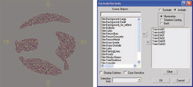
Figure 10-10. Illuminating 2D trees with 4 direct instanced lights.
The benefit of using this approach is striking. In the left image of Figure 10-11, the 2D tree is illuminated with one light that represents the sun in the scene. Notice how easy it is to tell that the tree is just an image. Even when using global illumination, this variation in illumination will almost always still exist. In the image on the right, the tree is not illuminated by a single light representing the sun, but rather by 4 instanced direct target lights placed evenly around the scene. This 2D tree looks much better because it’s illuminated evenly. With a forest of trees, a 3D version might take several hours to render, but the same trees in 2D could render in seconds and still look decent. As stated earlier, whether your vegetation is sufficient as 2D or whether it should be replaced by a 3D version depends on a lot of things, such as rendering time available, distance from the camera, camera movement, available RAM, etc. However, when you do decide to use 2D vegetation, you should always make sure they are evenly illuminated using this type of approach.
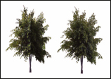
Figure 10-11. A 2D tree illuminated by a single shadow casting light (left) and 4 non shadow casting direct lights (right).
Creating Shrubs and Flowers
Another great landscaping application for the Scatter command involves creating the appearance of 3D shrubs and flowers over a large area in a very short amount of time. Besides scattering a tree over a surface, you can also scatter an individual face or a small number of faces over a volume. The face(s) you scatter, such as those shown in Figure 10-12, can be used to represent a leaf or a group of leaves and can be made to appear quite real at just about any distance as long as the leaf (or face) is not too large. Notice that there are three rows of the same images. The top row shows each leaf mapped on an individual face, while the 2nd and 3rd rows show the images mapped on 2 and 6 faces, respectively. Using a smaller number of faces for the scattered object means of course that the 3D vegetation you simulate will contain fewer faces. However, it also means that the shadows will be larger and less realistic. Notice also that mapping the leaves on objects with more faces such as the 3rd row means that the leaves can be shown larger. If the leaves can be shown larger, then you would need to use fewer of them to fill in a volume of space. If you need fewer objects, the result might actually be fewer total faces needed to fill a space. As you can see, choosing the object to scatter may take some experimentation.
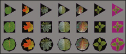
Figure 10-12. Faces that can be scattered about a volume to simulate realistic vegetation.
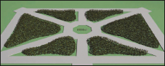
To create shrubs using this method, extrude a closed spline to the height you want to create your vegetation, and scatter the face(s) about this volume. To create the look of flowers among the shrubs, simply create a copy of the scattered leaves, raise the scatter slightly higher than the shrubs, reduce the number of duplicates as necessary to create the desired density, and apply a unique material that gives it a colored appearance as that of a flower. Figure 10-13 shows an image from an animation where this procedure was used to quickly populate a scene with shrubs and flowers. In this particular project, not only were landscape drawings not available, the client had absolutely no idea what they wanted for landscaping. As usual, the client said, ‘just make something that looks good’, and so this was our attempt to play the role of landscape architect.

Figure 10-13. Shrubs and flowers simulated by scattering faces within a volume.
The following exercise is a demonstration of the usefulness of the Scatter command in creating vegetation on a large scale very quickly. In this exercise, we will create vegetation in the rectangular garden area shown in Figure 10-13.
Creating Shrubs and Flowers
1. Open the file ch10-03.max.
2. Select the object Shrub-Area. This object consists of 6 closed splines, as shown in the next illustration. This will be the distribution object of the scatter and represents where the shrubs and flowers are going to be created.
3. Extrude the object 2’-0”. This will be the approximate height of the scattered object.
4. Select the object Leaf06small. This will be the leaf that is scattered about the volume just created. Notice that we are using the single faced version of this particular leaf.
5. Select Create > Geometry > Compound Objects > Scatter.
6. Click the Pick Distribution Object button and click on the object Shrub-Area.
7. In the Display rollout, enable the Hide Distribution Object option.
8. Select and delete the object Shrubs-Area.
9. In the Scatter Objects rollout, change the Duplicates value to 50,000.
10. Change the Vertex Chaos to 10.0. This helps break up the order of the scattered leaves.
11. In the Distribute Using section, enable the Area option.
12. In the Transforms rollout, use a value of 90 for each of the Rotation X, Y, and Z fields. This randomly rotates each face +/- 90 degrees about each axis. The result at this point should look like the next illustration.
13. Rename this object Site-Shrubs-Green.
14. Add the Edit Mesh or Edit Poly modifier to make the leaves on the faces visible in a shaded viewport.
15. Open the Material Editor.
16. Select the material Leaf06 and enable the Show Map in Viewport option. This cuts out the background of the leaf image.
17. Make a clone of this object and name it Site-Shrubs-Purple.
18. Change the Duplicates value of the Scatter object to 10,000. This makes the ratio of leaves to flowers, 5 to 1.
19. Move this object upward 12 inches.
20. Apply the material Leaf07. Notice that this material is nothing more than the same TGA file applied to the opacity channel but only a color for the Diffuse Color channel. Now you can change the color of this object by changing the diffuse color of the material. By doing so you can simulate the look of different flowers.
21. The result should look like the following illustration.

In this first part of the chapter, we looked at the differences between 2D and 3D vegetation and the many advantages and disadvantages of each. Additionally, we looked at a few tips and tricks for creating 2D vegetation. In the second half of this chapter, we will look at how to create realistic and efficient shadows for 2D vegetation, and finish by looking at ways to implement 3D vegetation effectively, without all the undesirable side effects that usually persist with their use.
Shadows for 2D Trees
Most objects you create for a visualization produce realistic shadows naturally. 2D trees, however, usually require additional work because they are nothing more than 2 criss-crossed polygons. Although creating realistic shadows can be quite a challenge, there are several techniques you can apply to vastly improve their appearance. The next portion of this chapter discusses four types of shadows that can be used in conjunction with 2D trees. Each has advantages and disadvantages and which method you use depends greatly on the same things discussed earlier: RAM, rendering time, distance from camera, etc.
Although there is no official title to any of these shadows types, we will use the following terms to delineate the different types:
• Opacity mapped shadows
• Image shadows
• 3D shadows
• Project light shadows
Opacity Mapped Shadows
Most shadow types allow you to use a map in the opacity channel to create the shadow of a tree, as shown in Figure 10-14. This option is automatically enabled for raytraced shadows and is also available for advanced raytraced shadows by enabling the Transparent Shadows option. The primary advantage of this particular shadow type is that it is very quick and easy to set up. By simply enabling an appropriate shadow type for a light, you can instantly create decent shadows with accurate placement. Notice in Figure 10-14 that the tree is perfectly aligned and positioned with the 2D trunk. This is often very difficult to achieve with the other shadow types.
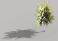
Figure 10-14. An example of opacity mapped shadows.
The primary disadvantage with this shadow type is the reduced shadow quality when lights are placed more directly overhead in a scene. Notice in the far left image of Figure 10-15 that the shadow looks fairly good, but in the other images the shadows become distorted as the sun moves higher and higher in the sky. If the sun were directly overhead, there would be no shadows cast at all (assuming the light was a direct light). When the sun is placed more than 60 degrees above the horizon, I wouldn’t even consider this shadow type to be an option. Because 60 degrees is our typical sun angle, this shadow type is our least favorite of the four options.

Figure 10-15. Opacity mapped shadows becoming more distorted with sun moving higher in sky.
Image Shadows
The quickest and least memory-consuming method of creating and rendering shadows for 2D trees is the Image Shadows method. You can literally add tens of thousands of these shadows with little more than a few seconds added to your rendering.
To use this method, create a polygon (2 faces), apply the image of a shadow to the polygon and place the polygon at the base of a tree. The grayscale image on the left side of Figure 10-16 is placed in the opacity channel on a material that is applied to a simple polygon.
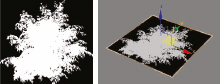
Figure 10-16. An example of image shadows.
When you render the image, the result appears to be a shadow whose color is determined by the diffuse color. Figure 10-17 shows 3 examples of variations in the diffuse color to simulate shadows of varying darkness.
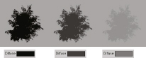
Figure 10-17. Changing shadow strength by changing the diffuse color.
And if you find that the shadows are too sharp, a simple adjustment of the Blur setting within the Coordinates rollout of the Opacity Map channel will give you the ability to soften the edges to your liking. Figure 10-18 shows some examples of adjustments to this setting. You can also achieve the results with a little more precision by adjusting the actual bitmap that is loaded in the opacity channel. The feather feature in Photoshop works great for making these adjustments.
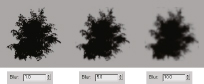
Figure 10-18. Changing shadow blurring by changing the Blur value in the opacity channel.
Once you have created your polygon and applied the material, place the polygon at the base of a tree, slightly above the ground object (1 inch usually works fine). Unfortunately, this shadow type doesn’t work well with 3D terrain because unless the ground around the base of a tree is completely flat, the 2D shadow object is likely to become at least partially buried in the ground. For 3D terrain, any of the other 3 shadow types would suffice.
Since all of your 2D trees that contain similar materials should be attached together (to prevent an unnecessary multitude of objects), image shadows that contain the same material should also be attached together. In fact, a nice trick to place this shadow type effectively is to attach a shadow to a 2D tree before you scatter the 2D tree. The result would be shadows that are always located in the proper place and a multi/sub-object material that controls both the tree and the shadow.
The last step is to turn off the Cast Shadows option for the object simulating shadows. When placing the image shadow for individual trees that are relatively close to the camera, it’s important to remember that the shadow must encompass the base of the trunk, as shown in Figure 10-19, otherwise the viewers will be left wondering why they can’t see the shadow of the trunk. It’s really not practical or necessary to worry about including a trunk in the shadow because then you will have to be meticulous in the placement of the shadow. In a forest of trees, you can speed up the process of creating shadows by scattering the polygon over a surface that defines the area where your trees are located. Accurate placement is rarely critical with a large number of randomly placed trees because you are usually viewing the shadows at a distance and/or the shadows of other trees are so close that they obscure any irregularities in placement.

Figure 10-19. Placing a shadow so it encompasses the trunk of a tree.
The speed at which these shadow types render is clearly their greatest advantage. But the greatest disadvantage is that they don’t cast accurate shadows. In Figure 10-20, the viewer would expect the shadow of the tree to fall on the object next to it, but instead the image shadow is obscured by the box.
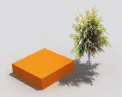
Figure 10-20. An image shadow does not fall on surrounding objects.
Another example of when this might become a problem is when you have a mulch bed with some minor relief. In the left image of Figure 10-21, the mulch bed rises about 6 inches above the ground, and therefore it doesn’t appear to receive any shadows by the image shadow object, which is only 1 inch above the ground. You could certainly raise the image shadow above the mulch, but doing so might make it obvious that the shadow is floating above the ground. On the other hand, if you’re so close that you can make this kind of distinction, you should probably try to use 3D trees or at least one of the better shadow types.
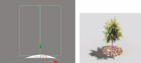
Figure 10-21. An example of how image shadows do not conform to 3D terrain.
One more important note about this shadow type is that you will almost always have to apply transparency to the shadow material so you can actually see the material of the object it appears to be casting shadows on. In the left image of Figure 10-22, you cannot see the grass through the image shadow. In the image on the right, the shadow is partially transparent, which enables the viewer to see the grass through the shadow. When you adjust the transparency of the image shadow, you will have to adjust the diffuse color of the shadow to account for the apparent change in color of the shadow.
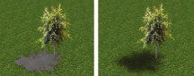
Figure 10-22. An image shadow without transparency (left) and with transparency (right).
For very fast and efficient renders, the image shadow simply can’t be beat. It’s not an exaggeration to say that the amount of time you save in the course of rendering, loading and saving files, and screen refreshes for a large project can be calculated in dozens of hours. For this reason, it is a great shadow type to implement in many situations.
3D Shadows
The most realistic type of shadow that can be used for a 2D tree is the shadow of a 3D tree. Unfortunately, it’s also the least efficient and most time-consuming method. To implement, simply place a 3D tree at the center of a 2D tree, disable the Visible to Camera and Visible to Reflection options of the 3D tree and disable the Cast Shadows option of the 2D tree. Figure 10-23 shows an example of a 2D tree using the shadow of a 3D tree. The 3D tree that was used was the Generic Oak from the 3ds Max Foliage feature. Even with the branches and trunk disabled, this particular tree can have from 5k to 8k faces, depending on which seed value you use. Although this is a relatively small number of faces for a scene with millions of faces, it might not be a good idea to use a large number of these trees to make 3D shadows because as few as 120 could add an additional one million faces to your scene.

Figure 10-23. An example of a 3D shadow with a 2D tree.
The disadvantages of this type of shadow are that it can drastically increase your rendering times and your scene file size, and can decrease your screen refresh rates if not used carefully. If you do decide to use 3D shadows, ensure that you use a tree with the minimum number of faces necessary to achieve the level of shadow detail needed. For example, the tree shown in Figure 10-23 contains over 5k faces and casts very nice shadows, but you can accomplish the same thing with a fraction of these faces. The tree shown in Figure 10-24 looks just as good but contains less than 500 faces. An easy way to create an object like this with fewer faces is to scatter a larger face about the volume of the higher polygon tree, using the higher polygon tree as a distribution object. For scenes with a large number of 3D shadow objects, the difference in rendering time, RAM consumption, and screen refreshes can be dramatic.
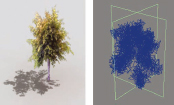
Figure 10-24. Scattering a larger face over the surface of a 3D tree to produce a low poly shadow.
Using such a small number of faces for a 3D shadow object might not be suitable for close-up views where a high level of shadow detail is needed; however, when such a high level of detail is needed in the shadows, it will also be needed in the visible tree itself. When this is the case, you shouldn’t be using a 2D tree anyway.
Another thing to remember when using 3D shadows with 2D trees is that even though the 3D shadow object has the Visible to Camera option disabled, it will still reflect light when you use global illumination. In fact, it will still reflect light when the Visible to Reflections option is disabled because this option has nothing to do with global illumination. Since the object still generates global illumination, it will significantly affect the color and highlights of the 2D trees. Therefore, you should consider giving the leaves of your invisible shadow object a particularly useful color. Figure 10-25 shows the effect of using different colors for the leaves of the 3D shadow object. This is a great way to create a varied look to a forest of 2D trees using the same image. You could actually make a significant improvement to a large group of trees by scattering different colored objects around the area of the trees and then making those objects invisible to a camera. The GI reflecting off those scattered objects would essentially paint the tree with different colors.
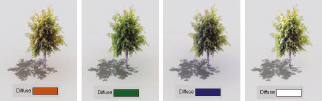
Figure 10-25. Using different colors on a 3D shadow to change the appearance of a 2D tree.
Finally, the reason the 3D shadow is the most realistic shadow type has little to do with the level of detail of the shadow. Other shadow types give you the ability to achieve the same level of detail without the negative side effects already discussed. What makes 3D shadows so great is that they cast correct shadows on surrounding objects, regardless of where the sun is placed in a scene.
Projector Light Shadows
In the Advanced Effects rollout of any light is the Projector Map feature, which allows you to use a light to project the image of a map or animation onto the surface of objects in your scene, as shown in Figure 10-26. The projector feature works the same way as a projector you would find in a movie theater, in which an image or animation is placed in front of a light and is projected onto a surface. But as you will see, this feature is also a great way to create realistic shadows for 2D trees.

Figure 10-26. An example of how the projector map channel of a light can be used.
Figure 10-27 demonstrates the use of a projector map to create a fake shadow for a 2D tree. The Cast Shadows option is disabled for the tree and the black-and-white image of the tree canopy (far-right image) is loaded into the projector map slot of the light, which is positioned just above the image of the tree. The multiplier of the projector light is then changed to –0.5, which causes light to be taken out of the area defined by the white portion of the tree canopy image. Negative multiplier values cause light to be removed from the objects hit by the light. The more negative the value, the darker the shadows.
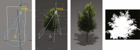
Figure 10-27. Using the projector map slot of a light to create the appearance of a shadow.
Although adding a large number of lights to your scene can drastically increase your render times, these types of lights render quickly because their effect is limited to a relatively small area. The primary advantage of this shadow type is the speed at which it renders and the ability to cast shadows correctly on 3D terrain and any surrounding objects. In Figure 10-28, you can see that the shadow is cast on the ground surface and on the surfaces of a nearby object. This effect is not possible with Image Shadows. In addition, the placement of the light doesn’t affect the quality of the shadows, and unlike opacity mapped shadows, you can have shadows created without any distortion; even when the light source is directly overhead.
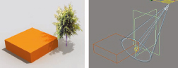
Figure 10-28. Projector lights casting shadows on a nearby object.
The greatest disadvantage to this shadow type is the multiplied effect of these shadows when they overlap each other. Notice in the left image of Figure 10-29 that there are two shadows and a darker area in the center. If each of these shadows were created using a -0.5 Multiplier value for the intensity the combined effect of both means that the area where the shadows overlap will have twice as much light taken away. So instead of the entire area of shadows having a multiplier value of -0.5, some parts in the center have a -1.0 value applied. In the image on the right, you can actually see three levels of shadow intensity because there are 3 overlapping project lights.

Figure 10-29. The combined effect of multiple shadows overlapping.
2D Trees in Action
To demonstrate the capability of the 2D tree in action, we have included a sample scene you can download and explore, labeled 2D_tree_animation.zip. A client had asked 3DAS to take their existing scene of a government facility, light it, create a 360 animation path and place trees around the perimeter of the property to give it a more natural and realistic surrounding. Because of the extremely tight deadline, we had no choice but to use 2D trees to speed the rendering process. Figure 10-30 shows two frames from this scene, with the government buildings omitted for privacy concerns. Because the scene was rendered in V-Ray, all V-Ray lights and materials have been removed and all of the vegetation has been converted to standard materials. By examining the scene, you will notice that all trees are 2D, all tree shadows are image shadows, and all the shrubs were created by scattering a single face. Because of the speed of the camera and the video filter used, it’s quite difficult for the viewer to discern that the trees are not 3D.
Notice the careful placement of the camera path and how during some parts of the path, trees in the foreground are just barely visible, as shown in the right image of Figure 10-30. Creating and finalizing the camera paths as early as possible is critically important to creating efficient scenes. Until the camera paths were finalized for this scene, we couldn’t finalize the placement of the trees. We wanted the tops of the trees in the foreground to be barely visible so the viewer would know that they were there but not see so much of them to know that they were 2D.
Finally, throughout the trees we scattered a single face to create the appearance of underbrush, which really added to the realism. Having a forest of trees can be made much more realistic when there is underbrush to break up the open look of flat terrain with a single texture.
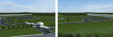
Figure 10-30. A example of 2D trees at work.
Creating 3D Trees
Adding 3D trees to your scene in a care-free manner can burden 3ds Max and your computer beyond their capabilities. Quite often, when you find that your computer runs out of memory or simply can’t complete a rendering in a reasonable amount of time, your vegetation is to blame. And the type of vegetation that can overburden your system quicker than any other is 3D vegetation. But fortunately, there are numerous tricks you can use to maximize the number of 3D trees your system will handle and minimize the amount of time it takes your system to render them. Let’s look at a few of them.
In the classes we teach at 3DAS, we find that even many experienced 3ds Max users don’t understand the significance of some fundamental optimization concepts. Students often ask us to look at their scenes and figure out why their rendering times are so excessive or why they run out of memory so quickly. So many users think that 4 GB of RAM or a top-end video card is needed on a regular basis when, in fact, it is not. So before going any further into a discussion on 3D trees, a little background on scene efficiency is needed.
Parametric vs. Editable
Parametric based objects are objects whose structure and appearance are dictated by parameters. Editable objects, such as the Editable Mesh and Editable Poly, are objects whose structure and appearance are dictated by the X, Y, Z values of location, orientation, and scale of the individual sub-objects that make up the objects. Parametric objects require very little data to store their existence, and therefore have a very small impact on a scene’s file size. The following discussion illustrates the important parts. Even when you apply modifiers and create compound objects out of parametric objects, the data for the object(s) is still stored parametrically.
If you save an empty scene with no objects in it, you will find that the file size is approximately 220KB (all of which is used to store system and file attributes). If you drop in a Generic Oak (from the 3ds Max Foliage feature) you will see that the tree contains approximately 25,000 faces. Saving the scene again causes the file size to increase to approximately 250KB. The reason for the small increase is that 3ds Max only has to store a small amount of data to represent this tree; such as X, Y, Z values, height, color, material IDs, etc. Now if you collapse this same tree into an editable mesh or poly and save the scene again, you will see that the file size has increased about six times to approximately 1.5MB. The reason is that this object’s geometry is no longer dictated by a small set of parameters, but rather by hundreds of thousands of values for the sub-objects that make up the editable object.
Collapsing an object to an editable mesh or poly should not be confused with simply adding the Edit Mesh or Edit Poly modifier. The differences between the two couldn’t be more significant and will be discussed later in Chapter 19. For now, an understanding of the previous two paragraphs is all that is needed.
Now clearly the Foliage feature in 3ds Max leaves a lot to be desired in terms of quality vegetation, but the concept of keeping vegetation parametric based rather than collapsing to an editable object is just as important for the many plug-ins that can be used to create vegetation. As an additional note, keeping plug-in based vegetation in parameter may be necessary just so you can take advantage of features, such as wind.
If you do have to use vegetation in editable form, ensure that duplicates are made as instances rather than copies. A forest of 3D instanced trees will have only a minor effect on file size, but the same forest of copied trees can result in ridiculous file sizes of several hundred megabytes.
Level of Detail
It’s always important to determine as early as possible where the final rendered views are going to be. By knowing this, you can determine the level of detail you will need from each view, and therefore, each tree. When creating vegetation, it’s critically important that you don’t use an excessive amount of indiscernible detail because doing so can quickly lead to excessive render times and memory consumption. To illustrate this, let’s look at the Generic Oak again.
As mentioned before, with the default values, the generic oak object contains approximately 25,000 faces, but if you disable just the branches of this object, the face count drops to approximately 7,000. Unless the view of a tree is very close-up, the viewer would most likely not even see a lack of branches. The standard 3ds Max foliage is certainly not something you should be using in production but the concept is still valid - reduce faces whenever possible. Quality vegetation software, such as Onyx, will allow you to turn off certain components such as branches, and set a polygon count limit so you can create very streamlined versions of your vegetation for situations where the vegetation is not so close to the camera.
The Almighty Proxy
A discussion about vegetation wouldn’t be complete without some mention of one of the best new features in 3ds Max 2009; the mental ray Proxy. This feature works much like an XRef, storing the data for an object in a separate file, thereby keeping your file sizes to a minimum. When you create a proxy, you are left with a facsimile display of the original object that is less of a burden to display, and therefore allows for easier and quicker viewport navigation. But the real benefit of the proxy lies in the way it allows you to conserve memory. Using proxies, you can render an entire forest of 3D trees without having to worry about running out of memory. The reason is because the proxy objects are treated as dynamic geometry as opposed to static geometry. Dynamic geometry is loaded and unloaded on the fly as needed, unlike static geometry, which is loaded at the start of a rendering and not unloaded until the rendering is completed. This feature alone makes using mental ray worthwhile. This feature has also been a part of V-Ray for several years and it works much the same way. If you use either mental ray or V-Ray, you should always consider creating proxies out of high-poly objects such as 3D trees.
Summary
Hopefully this chapter shed some light on the importance of creating efficient vegetation and some of the ways to create realistic looking vegetation without going beyond the capabilities of your computer. When done correctly, vegetation can be a simple element to create and not a menacing threat to your project’s success. These were just some of the many ways to implement vegetation efficiently and effectively. Your ability to find others is limited only by your imagination.