
CHAPTER 12
Global Illumination
ALTHOUGH THERE ARE NUMEROUS LIGHTING strategies within mental ray, it all boils down to understanding two essential methods of global illumination; Photon Mapping and Final Gathering. Each can be used independently of the other, or they can be used together to give even more lighting control. The key to using either of these methods is to understand the process. Once you understand what’s happening, you’ll understand what you can do to “tune out” the artifacts and “tune in” the solution. We’ll start with explaining photon mapping within mental ray.
Photon Maps
In real life, light sources emit infinite amounts of small energy packets called photons. These are the smallest quantifiable bits of energy that interact with their surroundings. Photons lose energy at a rate that is inversely proportional to the distance the photon travels from the light source and this can be expressed in the following equation, where x=distance from the light.
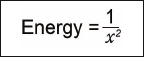
Figure 12-1. Inverse square law where x is the distance from the light source.
This decay is further compounded when they reflect and refract through various media further diminishing their energy. Unlike real life, when using mental ray we can discretely specify how many photons a light source will contribute, and define other properties such as how much energy a photon will have initially, how it will decay, and how it will interact with materials. Figure 12-2 illustrates the process.

Figure 12-2. Photon schematic diagram.
From the light source a photon is emitted with a specified energy. This photon interacts with a piece of geometry within the scene and leaves an imprint. It is then redirected via reflection or refraction depending on the material. During this interaction the photon has lost some of its energy and “picked up” some of the coloration of the material it interacted with (actually some frequencies are absorbed by the material giving the appearance of the photon picking up the surface color). This newly colored photon eventually interacts with another piece of geometry but since it has been colored from the last interaction, it imprints that color on the new geometry and is further tinted by the color of this new interaction. The new color of the photon is a blend of the first and second material color, which is a true physical phenomenon known as “color bleeding”. This process continues until a specified number of bounces are reached, or the photon is lost (no further geometry to interact with).
Let’s look at an exercise that demonstrates the use of photon mapping.
Using Photon Maps
1. Open the file Ch12-01.max. This is a very simple scene consisting of a white 20’x20’x9’ box with no openings, which therefore will prevent any photons from escaping. A light source is supplied by a standard spotlight at a height of 8’10” above the floor.

2. Open the Render Setup dialog and ensure that mental ray is your assigned rendering engine. The title of the Render Setup dialog will tell you this.
3. Click on the Indirect Illumination tab and scroll down to the Caustics and Global Illumination (GI) rollout. You’ll see two sections; one for caustic effects and another for global illumination (GI). We’re not generating any caustics for this scene so we don’t need to enable them, but we do need global illumination.
4. Enable Global Illumination (GI). The multiplier and color swatch are global settings that influence the initial intensity and color of photons and can be left alone for now. We’ll focus on the Trace Depth and Light Properties group and come back to the rest of the settings later.

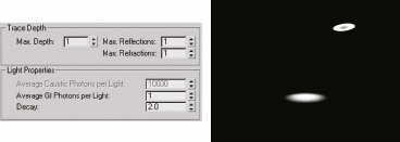
5. Set all the Trace Depth parameters to 1 and the Average GI Photons per Light to 1. This tells mental ray that we only want an average of 1 photon contributed by any single light in the scene.
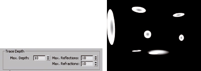
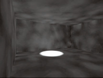
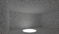
6. Render Camera01. The result should look like the following illustration. The spotlight is generating a pool of light on the floor as we would expect; however, you’ll notice the addition of another puddle of light that somewhat resembles a single white blood cell on the ceiling. This is mental ray’s way of depicting that a photon is being stored in this area of the scene. The photon was shot from the light source and was bounced off the floor to the ceiling where it stopped. This is because the photon was allowed one bounce since we set our Trace Depth to 1 (the lowest allowable setting).
7. Next, set all the parameters in the Trace Depth group to 2 and render again. Depending on your scene, you may or may not see another puddle of light. This is because the photon could be stored behind the camera outside our field of view.
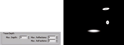
8. Increase all the Trace Depth values to 4 and render again.
9. Increase all the Trace Depth values to 6 and render again.

10. Increase all the Trace Depth values back to the default value of 10 and render again.
11. Set the Trace Depth parameters back to 5.
This brings up an important point that photons are view independent. So once we calculate a photon map, we don’t need to re-calculate it again should our view change. Because of this, we can save the photon map once and use it whenever we need to. Usually you would keep the Trace Depth numbers between 5 and 7 for most scenes. The only time you need to increase this value is when any single photon will have to travel through multiple transparent objects.
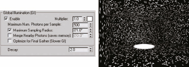
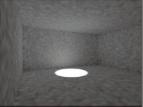
12. Increase the Average GI Photons per Light to 500 and render again. The result should look like the following illustration.
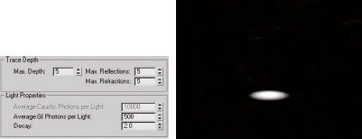
There are a couple of important things to note. The photon imprints (puddles of light) have lost their brightness making the rendering quite dark, and there is a lot of noise. The brightness issue is due to the fact that the photons share the overall initial energy. If we were to add more photons we would see an even darker image.
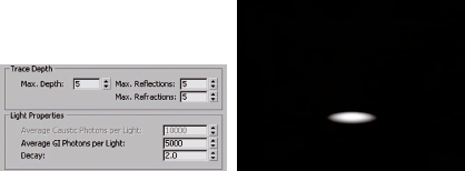
13. Increase the Average GI Photons per Light to 10,000 (the default) and render Camera01. The result should look like a darker version of the previous render. We have a couple of options to increase the light level. The first option is to increase the GI multiplier to a higher value, which will increase the photon energy.
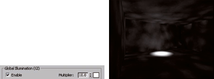
14. Increase the GI Multiplier to 10.0 and render again.
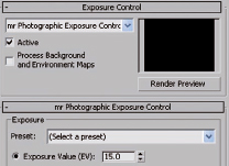
The second option is to use Exposure Controls to tone-map the rendered image using the new mr Photographic Exposure Control.
15. Turn the GI multiplier back to 1.0. On the menu bar go to Rendering > Exposure control, change the exposure control to mr Photographic Exposure Control.
16. Enable the Exposure Value (EV) option in the mr Photographic Exposure Control group, and press Render Preview.
17. Hold down the lower spinner arrow to lower the EV value, while you watch the Preview Render. The image will become visible near a value of -3.
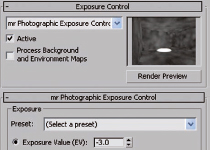
18. You can fine tune the number using keyboard entry. Exposure value is a simple way of controlling exposure with a single setting. Alternatively, you could adjust the exposure control via shutter speed, f-stop, and ISO values if you have an understanding of real world photography.
Once you like the illumination in the Render Preview, do the full size render. The noise will be tuned out later in this chapter and we’ll come back to the exposure control settings, but for now let’s continue with further GI adjustments.
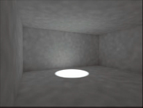
19. Back on the Render Setup dialog Indirect Illumination tab, within the Global Illumination section of the Caustics and Global Illumination (GI) rollout (not the Volumes section), enable the Maximum Sampling Radius and render again. This limits the size of the individual photon imprints to whatever radius we specify and with the default value of 1”, the result should look like the following image. If you don’t see anything, make sure your exposure control is set low enough.
Notice that since the photon imprints are smaller, they’ve become brighter since the same amount of energy is being distributed over a smaller area, making them appear more intense. If we don’t have this checkbox enabled, the photon imprints are defaulted to 1/10 of the overall scene dimensions (which in this scene would be 1/10 of 20’ or 2’ radius) This works fine for when we use photons in conjunction with final gather, but for photon-only solutions, we need to have enough photons to get detailed illumination within our scene (this can easily be in excess of several million photons). With that many photons, you couldn’t effectively have the photon imprints all at 1/10 of the scene size. The goal is to increase the size of the photon imprints to get them to just overlap, and then subsequently smooth out the solution by increasing the Maximum Number of Photons per Sample to something higher than the default 500.
20. Change the Average GI Photons per Light to 1,000,000 and render again. There is now little chance for any part of the scene to not be covered by a sample, but the image will look quite noisy.
21. Within the Global Illumination section (not the Volume section), change the Maximum Sampling Radius to 3” and render again.
22. By increasing the sampling radius we are filling in the spaces between the illuminated points, and increasing the chance of getting the photon puddles to overlap. By making the pools of illumination larger, we fill in these gaps in the illumination.
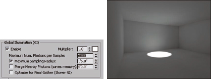
23. Change the Maximum Number of Photons per Sample to 6000 and then render. We’re telling mental ray to use a maximum of 6000 photons per sample, but we’ve got a small sampling radius. Increase the radius to 1’6” and render again. The result should look like the following illustration. Notice how the samples have been smoothed better than in any previous render.
The Maximum Number of Photons per Sample is of no real benefit, unless we have a dense population of photons to begin with. In this case we used approximately 1,000,000 photons so we could get away with a high number of photons per sample (in this case 6000). If we only had the default 10,000 photons we wouldn’t gain any benefit to using 6000 photons per sample since that is over half of the total amount of photons stored in the scene. These two values go hand in hand. The number of photons per sample is what we use to “tune out” the noisy artifacts associated with a photon only solution. It basically averages out the individual illumination values based on the number of photons sampled.
24. Change the Maximum Number of Photons per Sample back to the default 500 and render again. You see that since we’re averaging illumination levels across fewer photons, we end up with more noise.
As mentioned before, we can save and reuse a photon map.
25. In the Reuse FG and GI Caching rollout, find the Caustics and Global Illumination Photon Map section. Change the Dropdown menu from Off to Read/Write Photons to Map files. Click on the icon with three dots to the left of the text field, as shown in the following illustration. This will prompt you to store the photon map to a location you determine.
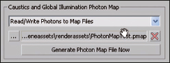
26. Specify a name and location to save the photon map.
27. Render out the scene and wait for the photon emission calculation to finish, or simply click the Generate Photon Map File Now button. Once done, your photon map is saved and ready to be re-used automatically. With a saved map, you won’t have to wait and go through the emission calculation stage every time you render. If you wish to resave another photon map, you can either specify another file name or click the Delete button to the right of the file name, and then recalculate another photon map.
Depending on how many photons you’re storing, your file sizes can get quite large. To help with this, mental ray has a new tool that will merge nearby photons. By enabling this tool we can set a radius that mental ray will use to merge nearby photons, thus optimizing the photon map.
28. Set the Average GI Photons per Light back down to 500, set the Maximum Sampling Radius to 6” and click Generate Photon Map Now again.
29. Enable Merge Nearby Photons (saves memory) and in the field immediately to the right, enter a value of 12”. The left image of the following illustration shows the photon map without this merge feature while the right shows the resulting map with this feature enabled.

Inverse Square Law
The last parameter to discuss in the Caustics and Global Illumination (GI) rollout is the Decay. Recall Figure 12-1, the equation for inverse square where the exponent shown in the formula is 2? This corresponds to the Decay value as shown in Figure 12-3.

Figure 12-3. Decay is set to the inverse square law exponent (2) by default.
If we were to set this parameter to 1, lights would have a linear falloff to their intensity rather than an exponential. This will allow the photons to lose their energy slowly and as a result, the scene will contain higher illumination values. Likewise, if we set this value to 3 we would have an inverse cube defining the decay. Simply put, values around 2 are physically accurate and anything else would not be. Values between 1 and 2 will allow the light to permeate deeper into the scene while values between 2 and 3 will darken a scene, since light will no longer be able to travel as far.
Another section of the Caustics and Global Illumination (GI) rollout not yet mentioned is the Volumes section. These settings control volumetric effects; however, there are other more practical methods for generating effects of this type and as such will not be covered here.
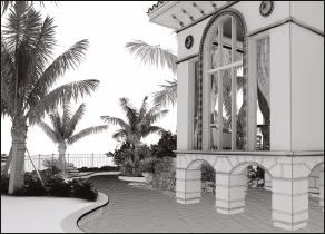
So why would you use photon mapping? As a rule of thumb, photon mapping is primarily used for interior scenes and usually in combination with final gather. The benefit of using photons to calculate GI is realized anytime you have a somewhat enclosed space with lots of artificial lighting. Photon mapping is typically not used for exterior daylight renderings because the photons will usually only bounce once or twice before being lost. Even if you surround the exterior scene with geometry like a sphere so as to trap the photons, the contribution to the final image quality is usually negligible and exterior GI can easily be accomplished by only using final gather.
Final Gather
Final gather can be looked at as the opposite method to photon mapping. Instead of shooting photons from a light source into the scene, sampling rays are shot from the camera into the scene, to sample the contribution of light on an object’s surface. Unlike photon mapping, this method is view dependent, meaning a new final gather map would need to be generated, or updated, if your view was to change. The process of incrementally adding samples to a final gather map is useful for creating animations and will be discussed later.
As mentioned, we are sending sampling rays from the camera into the scene. This means that a ray will sample a point on the surface of an object to see how much light is being contributed by its surroundings. The result is that we can use things like HDRIs, self-illuminated materials, photon maps, mr Physical Sky, and areas lit by lights to define the surface’s illumination. This process is similar to Ambient Occlusion, which will be discussed in the next chapter.
The Final Gather Process
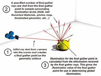
Figure 12-4. Creation of a final gather point.
The following is a summary of the final gather process shown in Figure 12-4:
• A single sampling ray is shot from the camera into the scene.
• This ray comes in contact with a piece of geometry in the scene.
• A final gather point is created on the surface of the geometry, much the same as what happens with a photon imprint.
• This final gather point then sends a specified number of final gather rays into the scene. Some rays will hit the surrounding geometry, some may be lost through a window, and some may hit an environment map (like the mr Physical Sky or HDRI files) or skylight. Either way, there may be a variety of samples taken for each final gather point.
• Mental ray then averages these sampled values to generate the illumination and color value of the final gather point. This information is then used at render time to calculate the illumination in the scene in a similar way to photon mapping. The main difference is we’re using final gather points instead of photon imprints.
Let’s look at an exercise that demonstrates the final gather process.
Using Final Gather
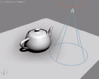
1. Open the file Ch12-02.max. This scene contains a plane, a teapot, and a spot light. The spotlight is intentionally missing the teapot because we’re expecting the final gather process to be able to see the puddle of light and determine how much this puddle is contributing to the surface illumination of the teapot.
2. Within the Indirect Illumination tab of the Render Setup dialog box, open the Final Gather rollout and enable Final Gather.
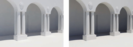
3. Using the Preset slider, select Draft and render Camera01. The left image of the following illustration shows the scene with final gather enabled and the right image shows the scene with final gather disabled. Note that the pool of light adds no secondary illumination with final gather disabled, but once final gather is enabled the surfaces of the teapot see the pool of light and provide secondary illumination for the teapot.

To better understand what is happening, we’ll take a look at what the final gather points look like.
4. Within the Processing tab of the Render Setup dialog box, open the Diagnostics rollout and select the Enable option.
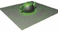
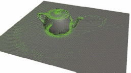
5. Select Final Gather from the list of diagnostics and render the scene again. The green dots are the individual final gather points. .

6. Return to the Final Gather rollout within the Indirect Illumination tab, set the Initial FG Point Density to 1 and re-render the scene. When we change the density to 1, the preset mode automatically changes to Custom. In draft mode we had an initial final gather point density of 0.1, and as shown in the previous illustration, the dots were relatively sporadic compared to what we have now with a density of 1. The denser these final gather points are, the greater the lighting detail will be but at a cost of longer render times.
Keep in mind that each of these final gather points is sampling the surrounding scene’s geometry and environment. More importantly, each of these final gather points is using the draft default Initial FG Point Density value of 50. This means that 50 rays are used with each point to sample the surroundings. This presents an opportunity to balance speed versus quality. If we want a higher final gather point density, we can offset the increase in rendering time by lowering the number of final gather rays cast by each point. If we have 100 final gather points in a scene with 50 final gather rays per point, then 5000 samples would be calculated, which is the same number of samples calculated if we have 1000 final gather points casting 5 final gather rays each. Of course the more final gather rays we cast, the better our solution will be, so you need to play with these values on a scene per scene basis.
Now we’ll take a closer look at the final gather settings.
7. Open ch12-3.max. Note that the following exercise uses a mr Daylight System. This type of lighting requires exposure control, so we need to enable this first.
8. Set exposure control to mr Photographic Exposure Control, then press Render Preview.
9. Within the mr Photographic Exposure Control rollout, click on the preset drop-down list and select Physically Based Lighting, Outdoor Daylight, Clear Sky. While watching the Render Preview window, make adjustments to the EV value, and the Image Control settings of Midtones, Shadows, and Highlights to best fit your monitor display.
10. Within the Indirect Illumination tab of the Render Setup dialog box, open the Final Gather rollout and take note of the values used for Initial FG Point Density, the Rays per FG Point, and Interpolate Over Num. FG Points. A very low density of 0.1 is used while only 1 ray per point is calculated and only 1 point is used in the interpolation process.
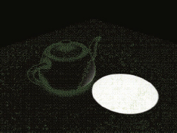
11. Render Camera view. The result should look like the following illustration. The cell-like appearance is mostly a result of the three values mentioned in the previous step. We have a low concentration of final gather points, each final gather point is only sending out one sampling ray, and we are not yet blending the final gather points together. You can see that some spots are black indicating that the single final gather ray wasn’t able to sample anything that had a luminance value.
12. Increase the Initial FG Point Density to 1 and render again. As you can see from the following illustration, we don’t necessarily get a better picture, but we do get more detail since we have a higher density of final gather points. To obtain a better solution we need to smooth out the illumination values. There are essentially two methods we can use. The first, and most obvious, is to use more final gather rays per sample. This will allow each final gather point to sample more of the surroundings, and hence obtain a smoother result.

13. Set the Initial FG Point Density back to 0.1, increase the Rays per FG Point to 50 and re-render. As the next illustration shows, this yields a closer approximation of luminance values from final gather point to final gather point, but we still see the individual samples. To get rid of this obvious delineation between final gather points, we’ll need to interpolate (or smooth) each sample with the surrounding samples. Before we do this let’s look at the other end of the spectrum.

14. Set the Rays per FG Point value back to 1 and change the Interpolate Over Num. FG Points from 1 to 30. Notice how the previous illustration and the following illustration both show a generally decent amount of illumination; however, the number of rays used in the previous illustration and the amount of interpolation used in the following illustration have to be used together before a decent solution can be reached.
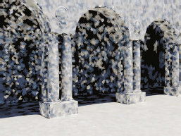
15. Set the FG preset back to Draft and render the scene. The following illustration shows how the solution is smoothed out by using 50 rays per FG point and then interpolating each point with the nearest 30 points. Although this gives us good results, you’ll notice that we’re lacking some detailed shadows. For us to get the detail we need to increase the final gather point density.
16. Increase the Initial FG Point Density to 1 and render the scene. This increased the shadow detail substantially, as can be seen in the middle columns and the doorway; however, the render time increased substantially. Even though we now have better shadow detail, we have introduced some noise to contend with. The noise is actually the detail being brought out. Incidentally, if you investigate the FG density values used for the Medium and High preset configurations, you would see that the 1.0 value we are using falls in between these presets.

At this point, we could interpolate over more points, but this would remove the shadow detail we gained with the increased FG point density. Instead, we’ll increase the number of final gather rays in hopes this will remove this noise.
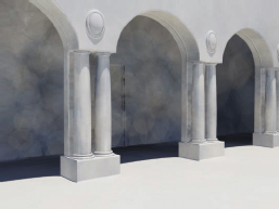
17. Increase the Rays per FG Point to 250 and render again. This removed the bulk of the noise, but there is still a residual amount left. We can continue to increase the Rays per FG Point in an effort to do this, but instead we’ll tune out the remaining noise with the interpolation setting.
18. Increase the Interpolate over Num. of FG Points to 50 and render again. Keep in mind that interpolation is blending final gather points, and by doing so, details can be lost if it is increased too high. This is similar to the blending method we employed with photon mapping in that if we have enough final gather points, we can have higher interpolation values. If you find that you need high interpolation values to get rid of the noise and as a result lose details, you can increase your density to get them back.

We can use a legacy feature called Use Radius Interpolation Method if we are unable to tune out noise and artifacts with the Interpolation Over Num. FG Points option. These are found just below in the FG Point Interpolation section.

Figure 12-5. Legacy method of interpolation as found in earlier versions of mental ray.
Typically, you should keep this to Radii in Pixels since this will then adaptively interpolate the fg points and will add any additional fg points at render time if needed. This means that final gather points can be created when needed. Be warned, if you have a low initial final gather point density and use this method, more final gather points will be created at render time, which can give you great results but with long render times. Through experience, I’ve found that enabling the maximum radius to 30 works well initially. Typically the minimum value should be 1/10 that of the maximum, so for a maximum of 30 pixels, the minimum should be set to 3 pixels.
Noise Filtering
There is another method to remove a noise with final gather; by using Noise Filtering within the Advanced section of the Final Gather rollout, as shown in Figure 12-6.
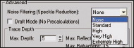
Figure 12-6. Noise Filtering dropdown menu.
By default this is set to Standard and I recommend that you start with this turned off (None) and increase as needed. This filter works in conjunction with the Rays per Final Gather Point value by filtering the samples collected from a single final gather point. If any of the final gather rays return a value that is significantly different to neighboring points, it will be rejected from the calculation. This way, the remaining usable samples for each final gather point will be within a defined threshold and will yield more consistent final gather point values. There is a downside, however. As you increase this filter from High to Very High to Extremely High, you remove GI data in the form of light rays and this will cause your scene to get progressively darker. The artifacts this filter removes are usually bright patches, as shown in Figure 12-7. You can easily see these if you turn interpolation off by setting the Interpolate Over Num. of FG Points to 1). If you see white splotches, you will need to use this filter.

Figure 12-7. Example of artifacts that Noise Filtering will aid in removing.
In the Basic section of the Final Gather rollout is a spinner field called Diffuse Bounces that allows the final gather rays to see beyond a single trace. This typically brightens up the image at the expense of greater color bleed, lower contrast, and longer rendering times. The color bleed and contrast can be tempered with the Weight parameter, but the higher render times cannot. The weight parameter will allow you to tell mental ray how much influence the diffuse bounces will have on the solution.
19. Set the final gather settings back to Draft.
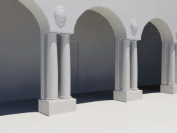
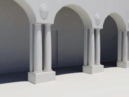
20. Change the Diffuse Bounces to 2 and render the scene. The result should look like the left image in the following illustration.
21. Change the Weight to 0.25 and render again. The image on the right shows the apparent increase in illumination, but is then tempered by the weighting to bring back the contrast as shown in the image on the right.
Saving the Final Gather Map for Animations
We can also save the final gather map, which is similar to the photon map; however, it’s important to understand that final gather maps are view dependent. This means that if our view changes, we’ll need to create a new map or when possible add more final gather points to the existing map.
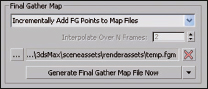
Figure 12-8. The Final Gather Map section.
22. Open up Ch12-4.max and render Camera01. The result is a diagnostics image as shown in the following illustration.
23. Within the Final Gather group of the Reuse (FG and GI Disk Caching) rollout of the Indirect Illumination tab, click on the icon with three dots, as shown in Figure 12-8, and choose a name and location to save the final gather map.
24. Render the scene to allow the final gather calculation to complete and allow the map to be saved. The result looks like the left image of the following illustration.
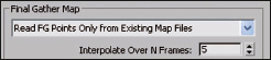
25. In the Final Gather Map group, click the dropdown arrow and change it to Read FG points Only from Existing Map Files. This prevents the FG map from being overwritten and keeps the previously saved map in place.
26. Switch to Camera02 and render this camera view. You’ll notice that there are no final gather points behind the teapot, as shown in the right image.

Before moving on I’d like to explain what is being seen. mental ray overlays the diagnostic final gather map at render time and does not occlude the fg points with the geometry. This means that the geometry will not hide the green dots that represent final gather points. Thus you’re able to see final gather points “through” the geometry in the scene, which can be confusing (such as the final gather points at the base of the teapot). The absence of points in certain regions is due to the creation of final gather points based on our last view. If we wish to add these points, we only need to choose Incremental Add FG Points option and render again from this new point of view.
27. From the dropdown list pick Incrementally Add FG Points to Map Files and re-render Camera02. You’ll notice that there is another final gather calculation phase and more final gather points are added to the existing final gather map.
Notice that new points are appended to the original map behind the teapot where none were found before.
So what does this mean to you? This is an important concept when doing architectural animations. Typically a camera is animated to move through the space, and as such ‘sees’ only select portions of the model. What we need to do is create final gather points on all the geometry the camera sees. Recall that I mentioned the final gather process is view-dependent. So this means that we only need to create final gather points on whatever the camera sees. Obviously, in an animation the view changes from frame to frame. As we’ve just seen, we can add final gather points to an existing final gather map quite easily. Theoretically, this means we could create a final gather map at frame 1, then add more points at frame 2, and so on. This is not a very economical way of doing it. Usually we can get away with rendering every 5th or 10th frame since there may be very little change from frame to frame. If your animation is slow, you can get away with a wider spacing (say every 30 frames) or if your camera is fast you would need narrower spacing (every second or third frame). For animations, you simply have to “see” all the geometry along your animation path.
It’s important to note that when you calculate a final gather map, you don’t need to render a production quality image. Thus, you can turn your sampling down to 1/64 for the max and min values to save time. As mentioned earlier, the frame spacing is determined by how fast your camera moves, and if you can “see” all the geometry along your animation path because final gather points are created based on your view. Also, you don’t need to save the final rendered image when calculating a Final Gather pass since this pass is only done to create a final gather map.
Once the final gather map is calculated we can render the final image sequence by enabling the Read FG Points Only from Existing Map Files option. Set your sampling back to production settings and set the renderer from rendering every nth frame to every 1th frame. This is usually overlooked and causes frustration. Now, render the image sequence as you normally would and mental ray will read the calculated final gather map for illumination levels and create the final rendered image.
If at any time you see some abnormal flickering occurring within your animation, check to see if the final gather map actually “saw” that geometry at that particular frame. If it didn’t, you need to unlock the Read Only (FG Freeze) option and append that frame to the final gather map and then re-render the troublesome frames. Note that you can also append final gather points by using the render region option to avoid rendering the entire frame when it wasn’t needed.
What it boils down to is that mental ray requires two stages for its GI. The first stage is the calculation of the lighting information via photon and/or final gather maps. Stage two is the rendering of the final image.
A special feature was added in 3ds Max 2009 to compensate for animation flicker caused by moving objects when using Final Gather maps. You can choose to create multiple final gather map files by going to the Mode group and choosing One File per Frame (Best for Animated Objects) and then interpolate between them using the Interpolate over Num Frames setting in the Final Gather Map group.

This addition to the Final Gather workflow provides precise control to eliminate troublesome image sections when animating. I won’t delve into it here, so if you need to use it, follow the procedures outlined in the 3ds Max Reference accessed through the Help menu.
Photon Mapping and Final Gather
Both methods of global illumination can be used independently of each other, but we can also use them in conjunction with one another. The order of calculations is first the photon map, then the final gather map. This order is always maintained because the Final Gather process uses the information generated by the photon map. When using both methods, it is advantageous to select the Optimize for Final Gather option in your photon mapping. This will allow the Final Gather process to be more efficient in reading the photon map.
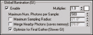
Figure 12-9. Optimize for Final Gather switch enabled.
If you’re wondering why would we want to use both methods, the simple answer is that photon mapping allows us to spray illumination throughout our scene based on the lights, and final gather uses this sprayed light in its calculations of GI. This results in better overall lighting. As stated before, this combination is best suited for interior scenes, scenes lit by artificial lights, or scenes that have deep niches that need illumination. We’ll end this chapter with a few helpful hints when using both methods of global illumination.
• You don’t require a large number of photons when using photon mapping and final gathering. Your photon map should have just enough photons to cover most of the geometry within your scene and you don’t need to specify a sampling radius.
• When rendering exteriors, you do not need a photon map. Final Gather when used in conjunction with a Skylight or mr Daylight System is your best option.
• When calculating your Final Gather map, you can get away with a smaller image size to minimize the render times. If your final output is say 640x480 pixels, you can render your Final Gather map at 400x300 (roughly 75% of the final output size).
• Final Gather can usually be set to Draft for most images. Detailed shadows can be more efficiently calculated using Ambient Occlusion, which will be discussed in the next chapter. If you choose not to use Ambient Occlusion, then higher quality final gather maps would need to be generated, which can add to your rendering time.
• Animations where objects are moving should not use photon mapping. Since photon mapping is view independent, if an object were to move, a new photon map would need to be calculated for each frame. A detailed photon map could take a long time to calculate and if this is done for each frame, render times will be unacceptable. Also, discrepancies from frame to frame can occur and give inadequate results. Instead, Final Gather can be used, or better yet, Final Gather with Ambient Occlusion should be used for animated objects.
Summary
In this chapter we’ve begun looking at the technical side of GI in mental ray. The important thing here is to understand the process to better know what needs to be done to eliminate any problems like noise, lack of detail, or artifacts. Knowing mental ray means knowing how to trouble-shoot.
Global illumination allows us to get realistic bounced light in the scenes but only gets us half way to photorealism. The other half comes from the materials we use in conjunction with GI. As just mentioned, ambient occlusion is a fast way to obtain the look of detailed GI solutions in a fraction of the time. Ambient occlusion, when used effectively, can be indistinguishable from detailed GI. We will look at this in the next chapter.