
CHAPTER 11
Introduction to mental ray
MENTAL RAY HAS MADE RECENT PROGRESS in the architectural arena since its first integration with 3ds Max in 1999. Perhaps in response to the success of Chaos Group’s Vray, Autodesk has added mental ray to its premier software programs, and now uses it as the core for materials in both Revit and 3ds Max. It is also the platform for the new iray renderer for 3ds Max 2012, a time-based rendering solution that offers a unique approach to image-making.
The power of mental ray was first acknowledged by Hollywood in 2003 with an Academy award presented to its creator, mental images. Earlier versions of mental ray found its way into visual effect studio pipelines where it was customized and tailored to the various studios’ needs. Autodesk saw the potential mental ray had as an alternative to scanline and radiosity, and as a render engine that could compete with new technology like Brazil, Final Render, and V-Ray. Now, with better documentation and a streamlined workflow, mental ray has found a home in many Autodesk products. The mental ray renderer offers powerful tools to create the most demanding visualizations and continues to become more accessible with each release. For many users, switching to a new rendering engine presents its challenges but understanding the basics goes a long way to flatten out the learning curve. We’re going to introduce some core concepts in this chapter that will prevent some pitfalls further down the road and get you up and running with mental ray so you can create stunning visualizations in very little time.
It’s worthwhile to note that although mental ray appears seamless within the interface, it still remains a separate rendering engine. Files are still translated and passed to mental ray for processing, although this is done transparently and is unnoticeable by the user. The translation process converts the scene into editable meshes, which is the native object type mental ray uses. This is important to know because it is highly beneficial to collapse your objects into editable meshes before you begin rendering as this will cut down the time taken for translation and ultimately allow for faster renderings.
As digital artists, we are constantly playing a delicate balancing act between rendering speed and rendering quality. To be effective at such a task, we need to understand some theory behind the complex mental ray render engine. We won’t be examining everything mental ray can do, but we will cover enough so you can feel comfortable with the program and be efficient with your work.
These chapters on mental ray are quite specific and the topics do not get into as much depth as may be needed for certain technical applications. Mental ray can be as complex as you want to make it and I would recommend getting a firm grasp on the concepts presented here as they create a strong foundation, and depict real-world use of the mental ray renderer. The topics discussed here can be applied to many applications that use mental ray and are not just limited to 3ds Max.
Whenever we do a rendering with mental ray, you’ll notice that the render proceeds via little white “bracketed” squares within the virtual frame buffer. These bracketed squares are called buckets and depending on how many processors, or the type of processor you have, you will see one or more buckets at a time rendering the final image. What we need to do is understand and optimize what’s happening within these buckets.
Image Sampling
The first concept we’re going to look at is Image Sampling, referred to in mental ray as Super Sampling. Image sampling is the technique of sampling beyond the resolution of the final image. This means that we can subdivide a pixel at render time to give it the proper coloration to avoid things like aliasing and loss of texture detail. This process doesn’t miraculously add more pixels, it simply allows the render engine to analyze a pixel more than one time and improve the final pixel color with each sampling pass. Mental ray is a super-sampler and gives us a lot of control over how it conducts the sampling.
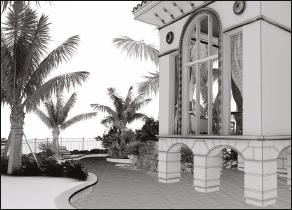
In Figure 11-1, notice that the sampling algorithm calculates the appropriate color of each rendered pixel. If we zoom in closely, you can see that the nice crisp edge is really just cleverly shaded pixels that give the illusion of a crisp edge.
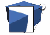
Figure 11-1. Example of anti-aliasing due to sampling.
To better understand how image sampling works, let’s take a look at a schematic grid of 9 pixels, as shown in Figure 11-2. For simplicity, we’ll look at the Fast Rasterizer sampling method, which takes samples at the center of each pixel or subpixel. The sampling method used when Fast Rasterizer is not enabled is more complicated but works on the same principles.
The individual squares in Figure 11-2 are representative of the individual pixels of a rendered image. The straight line traveling through the pixels represents an edge of the 3D box shown in Figure 11-1. Above the line is empty space (the white background) and below the line is the blue box. If we conduct one sample at the center of each pixel, as shown with the red dots in the left image of Figure 11-2, you can see that some samples “hit” the box while others miss. If a sample “hits” the box, the resulting pixel will be colored the same color as the box, or blue. If the sample “misses” the box, the resulting pixel will be colored the same as the background, or white.

Figure 11-2. Illustrating one sample per pixel and the resulting pixel shading.
Next we’ll super-sample the pixels. If we tell mental ray to divide each pixel into four subpixels and then take a sample at the center of each subpixel, it will have to do 4 times the work but will do a much better job at determining what color to assign each pixel to minimize artifacts such as aliasing, flickering, and swimming. To determine what final color a pixel should be, we only have to look at how many samples per pixel actually “hit” the box. If one of the four samples hits the box the resulting shade of the pixel would be a mixture of blue and white. If two of the four samples “hit” the box then the resulting shade of the pixel would be blue and white. The end result would be the right image of Figure 11-3.
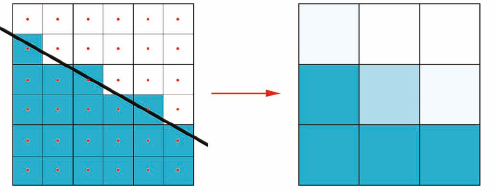
Figure 11-3. Illustrating four samples per pixel and the resulting pixel shading.
If we force mental ray to take 16 samples per pixel, the result would be an even better approximation, as shown in Figure 11-4.
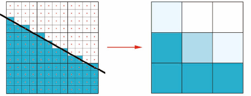
Figure 11-4. Illustrating 16 samples per pixel and the resulting pixel shading.
Keep in mind that we’re sub-dividing the pixels to get a better approximation of the final pixel color. Figure 11-4 still only represents 9 pixels, but we’ve illustrated each pixel undergoing 16 samples. Remember that the result is an averaging of color based on how many samples were blue and how many samples were white. So if 5 samples were white and 11 samples were blue, the resulting pixel color would be a blend of 5/16 white and 11/16 blue.
Obviously, the higher the numbers of samples per pixel, the better the approximation of the pixel color, but many more calculations are needed, which equates to longer render times. So why did we go through all this? We do this because of how mental ray deals with image quality. As mentioned previously, this is a simplified explanation. Mental ray can do intelligent sampling that is adaptive, or intuitive, based on the settings you dictate and the results determined from each pass. This means that mental ray can sample more when accuracy is needed and less when accuracy is not needed. This approach is effective for areas that lack detail or for large areas of smoothly shaded surfaces. This adaptive nature is the exact opposite of the technique known as the Brute Force method, by which every pixel is sampled the same amount. The downside to the brute force method is that it is not adaptive, which means you will do excessive calculations in areas of your image that don’t require them. By default, mental ray is automatically set to use adaptive sampling.
Image sampling is controlled most noticeably through the second and third rollouts in the Renderer tab of the Render Setup dialog box; Sampling Quality and Rendering Algorithms. Let’s first take a look at the Sampling rollout, shown in Figure 11-5. Here you can define the minimum and maximum number of samples to be taken per pixel. Whole numbers indicate how many samples will be taken per pixel. Fractional numbers indicate the number of pixels that will be grouped together to share one sample. For example, 1/4 means that only one sample will be taken for every four pixels. This is in essence the exact opposite of super sampling, but allows for very fast renderings when accuracy is not needed.
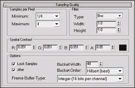
Figure 11-5. The Sampling Quality rollout.
For the sampling to be adaptive, the minimum and maximum values must differ and the more they differ, the more adaptive the image sampler is capable of being. By default the minimum sampling conducted is one sample for every four pixels and maximum sampling conducted is four samples per pixel. Mental ray will adaptively select how many samples are required based on the Spatial Contrast settings, which we will discuss a little later.
Recall that a higher sampling rate means more calculations and ultimately equates to longer render times. Although you can go as high as 1024 samples per pixel, it doesn’t mean you should. There are usually more efficient ways to smooth out aliased areas than using such high sampling. Usually you won’t need to go any higher than 16 samples per pixel. Figure 11-6 shows the effect of increased sampling from 1 sample for every 64 pixels (1/64) to 16 samples per pixel (16).

Figure 11-6. A Comparison of sampling rates; Top Left - 1/64, Top Middle - 1/16, Top Right 1/4, Lower Left - 1, Lower Middle - 4, Lower Right - 16.
Notice how each render is progressively more refined and that the increase in image quality starts to become less and less evident. The difference between 16 samples per pixel and 64 samples per pixel for this scene is negligible but rendering times are increased dramatically. As a rule of thumb you can keep the settings at min=1/4 max=4 for draft renders min=1 and max=16 for production renders. Sometimes you’ll find that you aren’t able to get acceptable results with the suggested production settings and think you can resolve them by choosing higher values. This is the wrong approach and should be avoided unless absolutely necessary. Instead you should try to employ the tools more efficiently to achieve the same improved results with less render time.
The adaptive image sampling process is driven by the parameters found in the Spatial Contrast section. The term Spatial Contrast can be reworded as ‘pixel variance’, which simply means the degree to which adjacent pixels differ in color. Lower values mean that pixels have to be more similar, or less spatially contrasted. If mental ray conducts the first pass of samples at the specified minimum rate and then determines from this first pass that two adjacent pixels are more spatially contrasted than is allowed by the Red, Green, Blue, and Alpha values another pass will be conducted at a higher sampling rate. Further passes will be conducted until the pixels meet these minimum criteria or until the maximum allowed sampling rate has been conducted. By lowering these values closer to zero, you’re forcing mental ray to use more maximum sampling rates, and by setting these values higher you’re allowing mental ray to use more of the minimum sampling rates. Essentially, if you use a value of zero, then you are telling mental ray you want perfect image sampling. Since this is not possible, the best it can do is use the maximum sampling allowed for every pixel, and this adaptive sampling method would essentially become a completely brute force method. Typically you should adjust these values together by using the color swatch shown in Figure 11-7 and then adjusting the Value setting. This in turn adjusts all the component values at the same time.
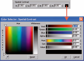
Figure 11-7. Spatial contrast settings and the Spatial Contrast color selector.
Jitter is an invaluable option for image sampling. It creates small perturbations in sampling at render time that will aid in smoothing out any aliasing issues that are still prevalent. This is one of the methods mentioned earlier that makes it possible to achieve higher quality renderings without having to rely so much on increasing the maximum image sampling rate. It is usually a good idea to enable this function whenever using mental ray, and Figure 11-8 shows a visual example of this effect.
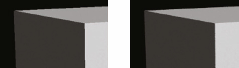
Figure 11-8. The effect of Jitter disabled (left) and enabled (right).
The last critical setting in this rollout is the Filter setting. Filters are basically algorithms that define the weighting for neighboring pixel blending. The filters increase in quality as you move down the list from Box, Gauss, Triangle, Mitchell, and Lanczos. The Box option is a good choice for draft renderings. Both Mitchell and Lanczos create varying degrees of edge enhancement and provide good choices for production still renderings. The Lanczos filter is much more exaggerated than Mitchell in the edge enhancement effect, but neither is suitable for animation because of the many types of artifacts they are almost guaranteed to create. Again, these include flickering, pixel dancing, pixel swimming, and numerous other terms associated with aliased images. A good choice for animations is the Gauss option with a Height and Width of 3, which would be similar to the Video and Soften filters. As you distribute the algorithm across more and more pixels, you create a softer image that becomes more and more blurred. It’s usually not a good idea to lower the default values.
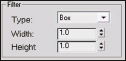
Figure 11-9. Filter settings used to smooth out image sampling results.
mental ray message window and BSP
An important tool to understand what is going on with the mental ray render engine is the mental ray Message Window, shown in Figure 11-10. This window gives us important information about our rendering such as render times, the rendering progress, any errors that occurred, etc. One of the most critical pieces of information we can track deals with a raytrace acceleration method known as BSP or Binary Space Partitioning.
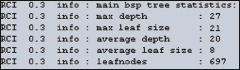
Figure 11-10. An excerpt from the mental ray Message Window showing average leaf depth and size.
Binary Space Partitioning is the method by which mental ray organizes a scene to conduct raytrace calculations. An easy way to think of this is placing a bounding box around your entire scene, and then cutting it up into cubes, or voxels, in such a way that each voxel contains a certain number of geometric triangles, as indicated by the Size value in the Raytrace Acceleration section of the Rendering Algorithms rollout. If a voxel contains more triangles than is specified by the Size the voxel is further split again. This splitting continues until the limit is reached, as dictated by the Depth. So in Figure 11-10 you can see that we continued to subdivide voxels to a maximum of 27 times. The average number of triangles contained in each voxel was 8. The average settings shown in Figure 11-11 are a good starting point to set your BSP leaf Size and Depth settings.
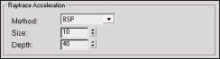
Figure 11-11. Binary Space Partitioning method.
Another raytrace acceleration method was introduced with 3ds Max 2009 known as BSP2. This method, now the default, automatically determines a proper size and depth value to use. This is a nice improvement but there are many situations in which you would benefit from using the older BSP method and adjusting these values manually. If you have the system resources available, you can increase rendering speed by setting your BSP depth to larger values and your size to lower values. Scenes heavily dependent on raytracing will definitely benefit from higher BSP depth settings. It’s important to know that if we increase the depth and decrease the size, we will improve render times but we’ll also be consuming a lot of additional resources. It’s better to start with the settings shown in the Message Window in Figure 11-10 and adjust them as necessary.
You should keep an eye on the max leaf size and average leaf size, as shown in Figure 11-10. If you see a large change in either of the two values away from the defaults, try increasing your average Depth value by 1. If the value is close to the initial size (in our case 8 and 21 as shown in Figure 11-10), you’re close to an optimal solution.
It’s worth mentioning here that if you are using 3ds Max 2008, you can often handle large scenes better by using the Large BSP option instead of the standard BSP method. This option is no longer available with 3ds Max 2009. Large BSP is suited for large scenes that tend to crash when rendered, which incidentally is much more likely on 32-bit computers and 32-bit 3ds Max. Large BSP will dynamically swap files to and from your hard drive, which can have a dramatic savings in RAM. This should be used only if you’re unable to render the scene due to memory issues because it is significantly slower than the BSP method. Regardless, the BSP or BSP2 methods are both good options with 3ds Max 2009 and later.
Distributive vs. Network Rendering
Distributive rendering is the ability to use processor cycles of networked machines to aid in the rendering process. This means that you can use multiple computers to generate the final rendered image, as long as they are part of the same local network. Note that this is different from network rendering, which sends out individual frames to networked computers. Network rendering is primarily used for creating animations, while distributed rendering is primarily used for creating stills. It’s important to note that network rendering with mental ray works seamlessly with Backburner.
Distributive rendering is enabled through the Distributed Bucket Rendering rollout of the Processing tab, as shown in Figure 11-12.

Figure 11-12. Distributive Rendering group.
Once distributed rendering is enabled, click the Add button and type a computer name or IP address of the computer you want included in the process. Unless you specifically want a special port, use the default port option.
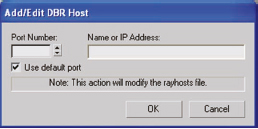
Figure 11-13. Distributive Bucket Rendering host window.
Continue to add up to 8 extra processors as necessary. Note that a dual core processor counts for 2 processor cycles. Additional processors can be purchased, but you don’t gain a substantial performance boost unless your network is incredibly fast. Also, depending on your firewall settings, you may have difficulty connecting to the satellite machines. If so, you may need a network administrator to set access for you. Be sure to enable Use Placeholder Objects option in the Translator Options when doing a distributive render. This will only send the geometry needed to render the view, rather than the entire scene. Once distributed rendering is set up, individual buckets are sent across the network and the final rendering is accomplished by several machines.
Summary
This chapter forms the foundation for establishing image quality and starts to introduce the concept of balancing image quality and rendering speed. This forms a base for us to build on in the following chapters. Many of the parameters we’ve adjusted in this chapter will need to be adjusted depending on the scene, and what works well for one rendering will not necessarily work well for the next. It is important to understand what the parameters do instead of arbitrarily relying on higher or lower values. Although the process can get quite technical, it’s the process that is most important to understand. From here we’ll look at how we can apply more technical parameters and use them to generate and tune global illumination within mental ray.