Chapter IA-3
Ideal Efficiencies
Chapter Outline
3. Efficiencies in Terms of Energies
4. Efficiencies Using the Shockley Solar Cell Equation
1 Introduction
In this chapter we deal with the simplest ideas that have been used in the past to attain an understanding of solar cell efficiencies from a theoretical point of view. The first and most obvious attack on this problem is to use thermodynamics, and we offer four such estimates in Section 2. Only the first of these is the famous Carnot efficiency. The other three demonstrate that one has more possibilities even within the framework of thermodynamics. To make progress, however, one has to introduce at least one solid-state characteristic, and the obvious one is the energy gap, Eg. That this represents an advance in the direction of a more realistic model is obvious, but it is also indicated by the fact that the efficiency now calculated is lower than the (unrealistically high) thermodynamic efficiencies (Section 3). In order to get closer to reality, we introduce in Section 4 the fact that the radiation is effectively reduced from the normal blackbody value (Equation (6)) owing to the finite size of the solar disc. This still leaves important special design features such as the number of series-connected tandem cells and higher-order impact ionisation, and these are noted in Section 5.
2 Thermodynamic Efficiencies
The formulae for ideal efficiencies of solar cells are simplest when based on purely thermodynamic arguments. We here offer four of these: they involve only (absolute) temperatures:
• Ta, temperature of the surroundings (or the ambient),
• Ts, temperature of the pump (i.e., the sun),
• Tc, temperature of the actual cell that converts the incoming radiation into electricity.
From these temperatures, we form the following efficiencies [1]:
![]() (1)
(1)
![]() (2)
(2)
![]() (3)
(3)
![]() (4)
(4)
In the latter efficiency, the cell temperature is determined by the quintic equation
![]() (5)
(5)
The names associated with these efficiencies are not historically strictly correct: for example, in Equations (2) and (3) other authors have played a significant part.
Figure 1 [1] shows curves of the four efficiencies, which all start at unity when Ta/Ts≡0, and they all end at zero when Ta = Ts. No efficiency ever beats the Carnot efficiency, of course, in accordance with the rules of thermodynamics. Values near Ts = 5760–5770 K seem to give the best agreement with the observed solar spectrum and the total energy received on Earth, but a less accurate but more convenient value of Ts = 6000 K is also commonly used. Using the latter value of Ts and Ta = 300 K as the temperature for Earth, one finds
![]()
If Ts = Ta = Tc one has in effect an equilibrium situation, so that the theoretical efficiencies are expected to vanish.
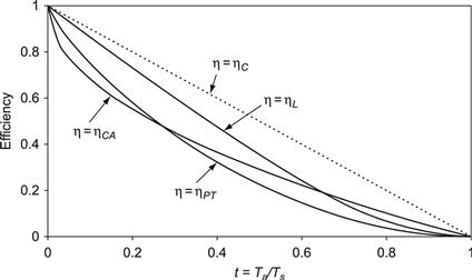
FIGURE 1 The efficiencies (1)–(4) as functions of Ta/Ts.
The above thermodynamic efficiencies utilise merely temperatures, and they lie well above experimental results. One needs an energy gap (Eg) as well to take us from pure thermodynamics to solid-state physics. Incident photons can excite electrons across this gap, thus enabling the solar cell to produce an electric current as the electrons drop back again. The thermodynamic results presented earlier, on the other hand, are obtained simply by considering energy and entropy fluxes.
3 Efficiencies in Terms of Energies
In order to proceed, we need next an expression for the number of photons in blackbody radiation with an energy in excess of the energy gap, Eg say, so that they can excite electrons across the gap. At blackbody temperature Ts the number of photons incident on unit area in unit time is given by standard theory as an integral over the photon energy [2]:
 (6)
(6)
Now suppose that each of these photons contributes only an energy equal to the energy gap to the output of the device, i.e., a quantity proportional to
 (7)
(7)
To obtain the efficiency η of energy conversion, we must divide this quantity by the whole energy that is, in principle, available from the radiation:
 (8)
(8)
Equation (8) gives the first of the Shockley–Queisser estimates for the limiting efficiency of a solar cell, the ultimate efficiency (see Figure 5). The argument neglects recombination in the semiconductor device, even radiative recombination, which is always present (a substance that absorbs radiation can always emit it!). It is also based on the blackbody photon flux (Equation (6)) rather than on a more realistic spectrum incident on Earth.
We shall return to these points in Section 4, but first a brief discussion of Equation (8) is in order. There is a maximum value of η for some energy gap that may be seen by noting that η = 0 for both xg = 0 and for xg very large. So there is a maximum efficiency between these values. Differentiating η with respect to xg and equating to zero, the condition for a maximum is
![]()
corresponding to η = 44%.
This is still higher than most experimental efficiencies, but the beauty of it is that it is a rather general result that assumes merely properties of blackbody radiation.
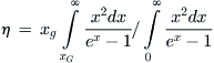
Let f(x) be a generalised photon distribution function; then a generalised efficiency can be defined by
 (9)
(9)
The maximum efficiency with respect to xg is then given by
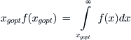 (10)
(10)
This is rather general and will serve also when the photon distribution departs from the blackbody forms and even for radiation in different numbers of dimensions.
4 Efficiencies Using the Shockley Solar Cell Equation
A further step in finding the appropriate efficiency limits for single-junction solar cells can be made by estimating the relevant terms in the Shockley ideal solar cell equation (Equation (1) in Chapter Ia-1). To this end, further remarks must be made about the solar spectrum and solar energy incident on Earth’s surface. The ultimate efficiency, discussed in Section 3, was based on the blackbody photon flux (Equation (6)), a rigorous thermodynamic quantity but not a very good estimate of the solar spectrum as seen on Earth. By virtue of the large distance between the Sun and Earth, the radiative energy incident on Earth’s surface is less than that of Equation (6) by a factor fω, which describes the size of the solar disk (of solid angle ωs) as perceived from Earth:
![]() (11)
(11)
where Rs is the radius of the Sun (696×103 km), and RSE is the mean distance between the Sun and Earth (149.6×10⁶ km), giving ωs = 6.85×10⁻⁵ sterad and fω = 2.18×10⁻⁵. The resulting spectrum is shown in Figure 2 alongside the standard terrestrial AM1.5 spectrum (a further discussion of the spectra that are used for solar cell measurements in practice can be found in Chapter III-2, which also shows the extraterrestrial spectrum AMO).

FIGURE 2 The blackbody spectrum of solar radiation and the AM1.5 spectrum, normalised to total irradiance 1 kW/m2, which is used for the calibration of terrestrial cells and modules.
The maximum value of the photogenerated current Iph now follows if we assume that one absorbed photon contributes exactly one electron to the current in the external circuit:
![]() (12)
(12)
where A is the illuminated area of the solar cell and q is the electron charge. The maximum photogenerated current density Jph = IPh/A that can be produced by a solar cell with band gap Eg is shown in Figure 3. To allow a comparison with photocurrents measured in actual devices, Figure 3 is plotted for the AM1.5 solar spectrum, which is used for calibration of terrestrial solar cells, rather than for the blackbody spectrum used in Section 3.
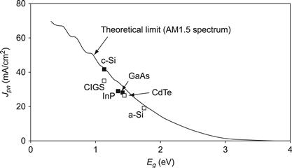
FIGURE 3 The theoretical limit on photogenerated current, compared with the best measured values. The curve is obtained by replacing the product fωΦ(Eg,Ts) in Equation (12) by the appropriate AM1.5 photon flux. Full symbols correspond to crystalline materials, open symbols to thin films.
The open-circuit voltage Voc can now be obtained using the photogenerated current Iph (Equation (12)) and the (dark) saturation current I0 that appears in the ideal solar cell equation:
![]() (13)
(13)
The current I0 can be obtained by a similar argument as the photogenerated current Iph, since, as argued by Shockley and Queisser, it can be equated to the blackbody photon flux at the cell temperature Tc (in what follows, the cell temperature Tc will be assumed to be equal to the ambient temperature Ta):
![]() (14)
(14)
where the coefficient f0 has been inserted to describe correctly the total area f0A exposed to the ambient photon flux. Various values of f0 (some dependent on the refractive index n of the cell material) can be found, appropriate for different device structures and geometries. The usual value is f0 = 2, as suggested by Shockley and Queisser [2], since this radiation is incident through the two (front and rear) surfaces of the cell. A similar argument for a spherical solar cell yields an effective value f0 = 4 [3]. Henry [4] gives f0 = 1+n2 for a cell grown on a semiconductor substrate, but the value f0 = 1 is also sometimes used (see, for example, [5]). Green [6] gives a semi-empirical expression for the dark saturation current density J0 = Io/A:
![]() (15)
(15)
An approximate analytical method for estimating Voc can also be useful, particularly as it stresses the thermodynamic origin of Voc. Indeed, it can be shown [7] that, near the open circuit, the solar cell behaves as an ideal thermodynamic engine with Carnot efficiency (1−Tc/Ts). Ruppel and Würfel [3] and Araùjo [8] show that Voc can be approximated to a reasonable accuracy by the expression
![]() (16)
(16)
which depicts the dependence of Voc on the band gap Eg and on the cell temperature Tc. Figure 4 compares this theoretical values for the open-circuit voltage with data for the best solar cells to date from different materials.

FIGURE 4 The theoretical Shockley–Queisser limit on open-circuit voltage: values exceeding this limit lie in the shaded area of the graph. Line corresponding to Equation (16) appears as identical to within the accuracy of this graph. Full symbols correspond to crystalline materials, open symbols to thin films.
Using now an expression for the fill factor (defined by Equation (3) in Chapter Ia-1), one readily obtains a theoretical estimate for the efficiency. Slightly different results may be encountered, principally by virtue of the different ways one can estimate the current and the voltage. Figure 5 shows the best-known result, the celebrated Shockley–Queisser ideal efficiency limit [2]. Shockley and Queisser call this limit the nominalefficiency, to be compared with the ultimate efficiency, which is discussed in Section 3. Figure 5 shows two such curves: one labelled ‘one-sun’ corresponds to the AMO solar intensity, as observed outside Earth’s atmosphere. A second curve, labelled ‘maximum concentration’ corresponds to light focused on the cell, by a mirror or a lens, at the maximum concentration ratio of l/fω = 45,872 [9].
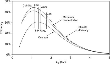
FIGURE 5 The ‘ultimate’ and two ‘nominal’ Shockley–Queisser efficiencies. Note that the blackbody radiation with temperature Ts = 6000 K has been used here, in keeping with the Shockley–Queisser work [2].
The various unavoidable losses in photovoltaic energy conversion by single-junction solar cells can be depicted in a graph constructed by Henry [4] and analogous to Figure 6. There are two curves in this graph:
• The photogenerated current density Jph from Equation (12) as a function of photon energy. Jph is divided here by the total irradiance, making the area under this curve equal to unity by construction.
• The maximum voltage that can be extracted from the cell at the maximum power point. This curve is drawn in such a way that the ratio of lengths of the two arrows b/a is equal to Vm/Eg.
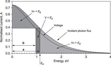
FIGURE 6 Henry’s construction.
The three shaded areas then depict the three fundamental losses in a single junction solar cell (shown here for silicon with band gap Eg equal to 1.12 eV):
• Shaded area marked hv < Eg is equal to the loss of current due to the inability of the semiconductor to absorb below-band-gap light.
• Shaded area marked hv > Eg represents energy losses due to the thermalization of electron–hole pairs to the band-gap energy.
• Hatched area marked V < Eg corresponds to the combined thermodynamic losses due to Voc being less than Eg and losses represented by the fill factor FF.
The area of the blank rectangle then represents the maximum efficiency that can be obtained for a single junction cell made from a semiconductor with band gap Eg. The graph is drawn here for light with maximum possible concentration. A different ‘voltage curve’ would result if light with one-sun intensity were used.
5 General Comments on Efficiencies
The ideal solar cell efficiencies discussed above refer to single-junction semiconductor devices. The limitations considered in the ultimate efficiency of Section 3 are due to the fact that the simplest semiconductor (i.e., one whose defects and impurities can be ignored) cannot absorb below-band-gap photons. Furthermore, it is also due to the fact that the part of the energy of the absorbed photons in excess of the band gap is lost as heat. Radiative recombination at the necessary fundamental level was taken into account in the treatment of Section 4. It is sometimes argued that there are other ‘unavoidable’ losses due to electronic energy transfer to other electrons by the Auger effect (electron–electron collisions) [10–12]. There is also the effect of band-gap shrinkage, discussed in Chapter Ia-2, and light trapping may also play a part [11]. None of these effects are discussed here, and the reader is referred to the relevant literature.
It is clear that it is most beneficial if one can improve the effect of a typical photon on the electron and hole density. This can be achieved, for example, if the photon is energetic enough to produce two or more electron–hole pairs. This is called impact ionisation and has been studied quite extensively. A very energetic photon can also project an electron high enough in to the conduction band so that it can, by collision, excite a second electron from the valence band. This also improves the performance of the cell. On the other hand, an electron can combine with a hole, and the energy release can be used to excite a conduction-band electron higher into the band. In this case, energy is uselessly dissipated with a loss of useful carriers and hence of conversion efficiency. This is one type of Auger effect. For a survey of these and related effects, see [12]. These phenomena suggest a number of interesting design problems. For example, is there a way of limiting the deleterious results of Auger recombination [13]? One way is to try to ‘tune’ the split-off and the fundamental band gaps appropriately. If one is dealing with parabolic bands, then the obvious way is to examine the threshold energies that an electron has to have in order to jump across the gap and make these large so as to make this jump difficult.
Then there is the possibility of placing impurities on the energy band scale in such a way as to help better use to be made of low-energy photons, so that they can now increase the density of electrons in the system. This is sometimes referred to as the impurity photovoltaic effect. So one can make use of it [14].
One can also utilise excitons to improve the efficiencies of solar cells. There may be as many as 1017 cm−3 excitons in silicon at room temperature. If they are split up in the field of a p–n junction, this will increase the concentration of current carriers and so increase the light generated current, which is of course beneficial.
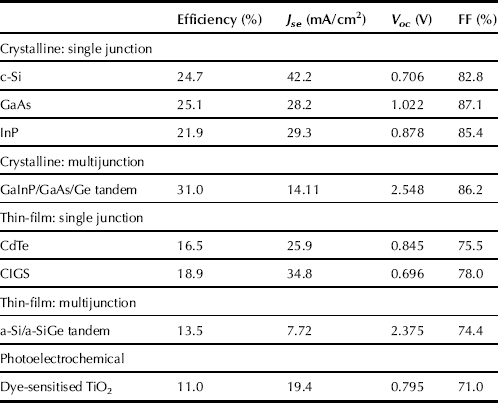
We have here indicated some useful ideas for improving solar cells, There are of course many others, some of which are discussed in Chapters Ib-2 and Id-2 as well as elsewhere [15]. Note, in particular, the idea of developing tandem cells in which photons hit a large band-gap material first and then proceed gradually to smaller band-gap materials. Tandem cells are now available with three of more stages. Solar cells with efficiency of order 20% arc predicted to be produced on a large scale in the near future [16]. Table 2 shows the best laboratory efficiencies at the present time for different materials.
TABLE 1 The Maximum Efficiencies of Tandem Cells as a Function of the Number of Cells in the Stack for Different Concentration Ratios [17]. Note that de Vos [17] Uses a Slightly Smaller Value of fω than Shockley and Queisser, Resulting in a Marginally Different Maximum Concentration Ratio than used in Figure 5
| Concentration ratio | Number of cells in the stack | Maximum efficiency (%) |
| 1 | 1 | 31.0 |
| 2 | 49.9 | |
| 3 | 49.3 | |
| … | ||
| ∞ | 68.2 | |
| 46.300 | 1 | 40.8 |
| 2 | 55.7 | |
| 3 | 63.9 | |
| … | ||
| ∞ | 86.8 |
TABLE 2 The Best Reported Efficiencies, at Time of Writing, for Different Types of Solar Cells [18]
References
1. Landsberg PT, Badescu V. Solar energy conversion: list of efficiencies and some theoretical considerations. Prog Quantum Electron. 1998;22:211–231.
2. Shockley W, Queisser HJ. Detailed balance limit of efficiency of pn junction solar cells. J. Appl Phys. 1961;32:510.
3. Ruppel W, Würfel P. Upper limit for the conversion of solar energy, IEEE Trans. Electron Dev ED. 1980;27:877.
4. Henry CH. Limiting efficiencies of ideal single and multiple energy gap terrestrial solar cells. J Appl Phys. 1980;51:4494.
5. Kiess H, Rehwald W. On the ultimate efficiency of solar cells. Solar Energy Mater Solar Cells. 1995;38(55):45.
6. Green MA. Solar Cells. New York: Prentice Hall; 1982;.
7. Baruch P, Parrott JE. A thermodynamic cycle for photovoltaic energy conversion. J Phys D: Appl Phys. 1990;23:739.
8. Araùjo GL. Limits to efficiency of single and multiple band gap solar cells. In: Luque A, Araùjo GL, eds. Physical Limitations to Photovoltaic Energy Conversion. Bristol: Adam Hilger; 1990;:106. .
9. Welford WT, Winston R. The Physics of Non-imaging Concentrators. New York: Academic Press; 1978; (Chapter 1).
10. Green MA. Limits on the open-circuit voltage and efficiency of silicon solar cells imposed by intrinsic Auger process. IEEE Trans Electron Dev ED-31 1984;671.
11. Tiedje T, Yablonovich E, Cody GC, Brooks BC. Limiting efficiency of silicon solar cells. IEEE Trans Electron Dev ED-31 1984;711.
12. Landsbcrg PT. The band-band Auger effect in semiconductors. Solid-State Electron. 1987;30:1107.
13. Pidgeon CR, Ciesla CM, Murdin BN. Suppression of nonradiative processes in semiconductor mid-infrared emitters and detectors. Prog Quantum Electron. 1997;21:361.
14. Kasai H, Matsumura H. Study for improvement of solar cell efficiency by impurity photovoltaic effect. Solar Energy Mater Solar Cells. 1997;48:93.
15. Green MA. Third generation photovoltaics: Ultra high conversion efficiency at low cost. Prog Photovoltaics Res Appl. 2001;9:123–135.
16. Wileke GP. The Frauenhoffer ISE roadmap for crystalline silicon solar cell technology. New Orleans: Proc. 29th IEEE Photovoltaic Specialists Conf.; 2002.
17. deVos A. Detailed balance limit of the efficiency of tandem solar cells. J Phys D: Appl Phys. 1980;13:839 (See also A. deVos, Endoreversible Thermodynamics of Solar Energy Conversion, Oxford University Press, 1992).
18. Green MS, K.I Emery, King DI, Igari S, Warta W. Solar cell efficiency tables (version 20). Prog Photovoltaics Res Appl. 2002;10:355–360.