
The exponential distribution is a special case of the gamma distribution, which we will also encounter in this chapter. The exponential distribution can be used to analyze extreme values for rainfall. It can also be used to model the time it takes to serve a customer in a queue. For zero and negative values, the probability distribution function (PDF) of the exponential distribution is zero. For positive values, the PDF decays exponentially:

We will use rain data as an example, which is a good candidate for an exponential distribution fit. Obviously, the amount of rain cannot be negative and we know that heavy rain is less likely than no rain at all. In fact, a day without rain is very likely.
The following steps fit the rain data to the exponential distribution:
- The imports are as follows:
from scipy.stats.distributions import expon
import matplotlib.pyplot as plt
import dautil as dl
from IPython.display import HTML
- I made a wrapper class that calls the
scipy.stats.exponmethods. First, call thefit()method:rain = dl.data.Weather.load()['RAIN'].dropna() dist = dl.stats.Distribution(rain, expon) dl.options.set_pd_options() html_builder = dl.report.HTMLBuilder() html_builder.h1('Fitting Data to the Exponential Distribution') loc, scale = dist.fit() table = dl.report.DFBuilder(['loc', 'scale']) table.row([loc, scale]) html_builder.h2('Distribution Parameters') html_builder.add_df(table.build()) - The following code calls the
scipy.stats.expon.pdf()method and thescipy.stats.describe()function on the fit residuals:pdf = dist.pdf(loc, scale) html_builder.h2('Residuals of the Fit') residuals = dist.describe_residuals() html_builder.add(residuals.to_html()) - To evaluate the fit, we can use metrics. Compute fit metrics with the following code snippet:
table2 = dl.report.DFBuilder(['Mean_AD', 'RMSE']) table2.row([dist.mean_ad(), dist.rmse()]) html_builder.h2('Fit Metrics') html_builder.add_df(table2.build()) - Plot the fit and display the analysis report as follows:
plt.hist(rain, bins=dist.nbins, normed=True, label='Rain')
plt.plot(dist.x, pdf, label='PDF')
plt.title('Fitting to the exponential distribution')

# Limiting the x-asis for a better plot
plt.xlim([0, 15])
plt.xlabel(dl.data.Weather.get_header('RAIN'))
plt.ylabel('Probability')
plt.legend(loc='best')
HTML(html_builder.html)
Refer to the following screenshot for the end result (the code is in the fitting_expon.ipynb file in this book's code bundle):
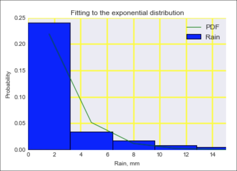
The scale parameter returned by scipy.stats.expon.fit() is the inverse of the decay parameter from (3.1). We get about 2 for the scale value, so the decay is about half. The probability for no rain is therefore about half. The fit residuals should have a mean and skew close to 0. If we have a nonzero skew, something strange must be going on, because we don't expect the residuals to be skewed in any direction. The
mean absolute deviation (MAD) and root mean square error (RMSE) are regression metrics, which we will cover in more detail in Chapter 10, Evaluating Classifiers, Regressors, and Clusters.
- The exponential distribution Wikipedia page at https://en.wikipedia.org/wiki/Exponential_distribution (retrieved August 2015)
- The relevant SciPy documentation at http://docs.scipy.org/doc/scipy-dev/reference/generated/scipy.stats.expon.html (retrieved August 2015)