
Mean, variance, skewness, and kurtosis are important quantities in statistics. Some of the calculations involve sums of squares, which for large values may lead to overflow. To avoid loss of precision, we have to realize that variance is invariant under shift by a certain constant number.
When we have enough space in memory, we can directly calculate the moments, taking into account numerical issues if necessary. However, we may want to not keep the data in memory because there is a lot of it, or because it is more convenient to calculate the moments on the fly.
An online and numerically stable algorithm to calculate the variance has been provided by Terriberry (Terriberry, Timothy B. (2007), Computing Higher-Order Moments Online). We will compare this algorithm, although it is not the best one, to the implementation in the LiveStats module. If you are interested in improved algorithms, take a look at the Wikipedia page listed in the See also section.
Take a look at the following equations:
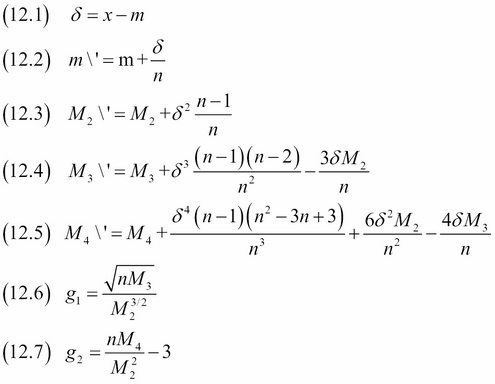
Skewness is given by 12.6 and kurtosis is given by 12.7.
Install LiveStats with the following command:
$ pip install LiveStats
I tested the code with LiveStats 1.0.
- The imports are as follows:
from livestats import livestats
from math import sqrt
import dautil as dl
import numpy as np
from scipy.stats import skew
from scipy.stats import kurtosis
import matplotlib.pyplot as plt
- Define the following function to implement the equations for the moments calculation:
# From https://en.wikipedia.org/wiki/ # Algorithms_for_calculating_variance def online_kurtosis(data): n = 0 mean = 0 M2 = 0 M3 = 0 M4 = 0 stats = [] for x in data: n1 = n n = n + 1 delta = x - mean delta_n = delta / n delta_n2 = delta_n ** 2 term1 = delta * delta_n * n1 mean = mean + delta_n M4 = M4 + term1 * delta_n2 * (n**2 - 3*n + 3) + 6 * delta_n2 * M2 - 4 * delta_n * M3 M3 = M3 + term1 * delta_n * (n - 2) - 3 * delta_n * M2 M2 = M2 + term1 s = sqrt(n) * M3 / sqrt(M2 ** 3) k = (n*M4) / (M2**2) - 3 stats.append((mean, sqrt(M2/(n - 1)), s, k)) return np.array(stats) - Initialize and load data as follows:
test = livestats.LiveStats([0.25, 0.5, 0.75]) data = dl.data.Weather.load()['TEMP']. resample('M').dropna().values - Calculate the various statistics with LiveStats, the algorithm mentioned in the previous section, and compare with the results when we apply NumPy functions to all the data at once:
ls = [] truth = [] test.add(data[0]) for i in range(1, len(data)): test.add(data[i]) q1, q2, q3 = test.quantiles() ls.append((test.mean(), sqrt(test.variance()), test.skewness(), test.kurtosis(), q1[1], q2[1], q3[1])) slice = data[:i] truth.append((slice.mean(), slice.std(), skew(slice), kurtosis(slice), np.percentile(slice, 25), np.median(slice), np.percentile(slice, 75))) ls = np.array(ls) truth = np.array(truth) ok = online_kurtosis(data) - Plot the results as follows:
dl.options.mimic_seaborn()
cp = dl.plotting.CyclePlotter(plt.gca())
cp.plot(ls.T[0], label='LiveStats')
cp.plot(truth.T[0], label='Truth')
cp.plot(data)
plt.title('Live Stats Means')
plt.xlabel('# points')
plt.ylabel('Mean')
plt.legend(loc='best')

plt.figure()

mses = [dl.stats.mse(truth.T[i], ls.T[i])
        for i in range(7)]
mses.extend([dl.stats.mse(truth.T[i], ok[1:].T[i])
             for i in range(4)])
dl.plotting.bar(plt.gca(),
                ['mean', 'std', 'skew', 'kurt',
                 'q1', 'q2', 'q3',
                 'my_mean', 'my_std', 'my_skew', 'my_kurt'], mses)
plt.title('MSEs for Various Statistics')
plt.ylabel('MSE')
Refer to the following screenshot for the end result:
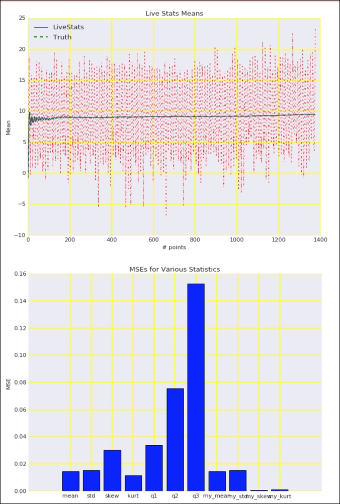
The code is in the calculating_moments.ipynb file in this book's code bundle.
- The LiveStats website at https://bitbucket.org/scassidy/livestats (retrieved January 2016)
- The related Wikipedia page at https://en.wikipedia.org/wiki/Algorithms_for_calculating_variance (retrieved January 2016)