The mean squared error (MSE) and median absolute error (MedAE) are popular regression metrics. They are given by the following equations:

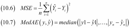
The MSE (10.6) is analogous to population variance. The square root of the MSE (RMSE) is, therefore, analogous to standard deviation. The units of the MSE are the same as the variable under analysis—in our case, temperature. An ideal fit has zero-valued residuals and, therefore, its MSE is equal to zero. Since we are dealing with squared errors, the MSE has values that are larger or ideally equal to zero.

The MedAE is similar to the MSE, but we start with the absolute values of the residuals, and we use the median instead of the mean as the measure for centrality. The MedAE is also analogous to variance and is ideally zero or very small. Taking the absolute value instead of squaring potentially avoids numerical instability and speed issues, and the median is more robust for outliers than the mean. Also, taking the square tends to emphasize larger errors.

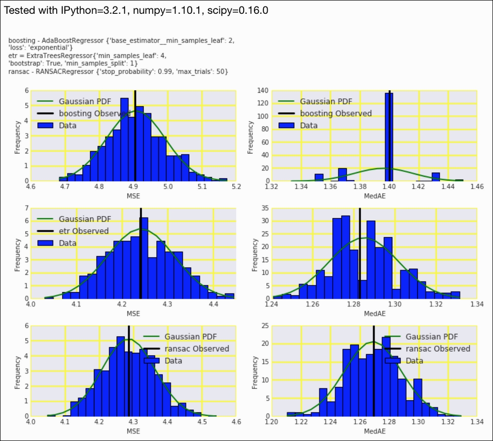
In this recipe, we will plot bootstrapped populations of MSE and MedAE for the regressors from Chapter 9, Ensemble Learning and Dimensionality Reduction.

How to do it...

1. The imports are as follows:

   from sklearn import metrics
   import ch10util
   from IPython.display import HTML
   import dautil as dl
   from IPython.display import HTML

2. Plot the distributions of the metrics for the temperature predictors:

   sp = dl.plotting.Subplotter(3, 2, context)
   ch10util.plot_bootstrap('boosting',
                           metrics.mean_squared_error, sp.ax)
   sp.label()
   
   ch10util.plot_bootstrap('boosting',
                           metrics.median_absolute_error, sp.next_ax())
   sp.label()
   
   ch10util.plot_bootstrap('etr',
                           metrics.mean_squared_error, sp.next_ax())
   sp.label()
   
   ch10util.plot_bootstrap('etr',
                           metrics.median_absolute_error, sp.next_ax())
   sp.label()
   
   ch10util.plot_bootstrap('ransac',
                           metrics.mean_squared_error, sp.next_ax())
   sp.label()
   
   ch10util.plot_bootstrap('ransac',
                           metrics.median_absolute_error, sp.next_ax())
   sp.label()
   sp.fig.text(0, 1, ch10util.regressors())
   HTML(sp.exit())

Refer to the following screenshot for the end result:

The code is in the mse.ipynb file in this book's code bundle.