

i
i
i
i
i
i
i
i
9.4. Signal Processing for Images 215
To work out the algorithmic details it’s simplest to drop down to 1D and dis-
cuss resampling a sequence. The simplest way to write an implementation is in
terms of the reconstruct function we defined in Section 9.2.5.
function resample(sequence a, float x
0
, float Δx,intn, filter f)
create sequence b of length n
for i =0to n − 1 do
b[i]=reconstruct(a, f, x
0
+ iΔx)
return b
The parameter x
0
gives the position of the first sample of the new sequence in
terms of the samples of the old sequence. That is, if the first output sample falls
midway between samples 3 and 4 in the input sequence, x
0
is 3.5.
This procedure reconstructs a continuous image by convolving the input se-
quence with a continuous filter and then point samples it. That’s not to say that
these two operations happen sequentially—the continuous function exists only in
principle and its values are computed only at the sample points. But mathemati-
cally, this function computes a set of point samples of the function af.
This point sampling seems wrong, though, because we just finished saying
that a signal should be sampled with an appropriate smoothing filter to avoid
aliasing. We should be convolving the reconstructed function with a sampling
filter g and point sampling g(fa). But since this is the same as (gf) a,
we can roll the sampling filter together with the reconstruction filter; one convo-
lution operation is all we need (Figure 9.38). This combined reconstruction and
sampling filter is known as a resampling filter.
reconstruct
sample
smooth
(f
r
f
s
)
f
r
f
s
Figure 9.38. Resampling involves filtering for reconstruction and for sampling. Since two
convolution filters applied in sequence can be replaced with a single filter, we only need one
resampling filter, which serves the roles of reconstruction and sampling.
i
i
i
i
i
i
i
i
216 9. Signal Processing
When resampling images, we usually specify a source rectangle in the units of
the old image that specifies the part we want to keep in the new image. For exam-
ple, using the pixel sample positioning convention from Chapter 3, the rectangle
we’d use to resample the entire image is (−0.5,n
old
x
− 0.5) × (−0.5,n
old
y
− 0.5).
Given a source rectangle (x
l
,x
h
) × (y
l
,y
h
), the sample spacing for the new im-
age is Δx =(x
h
− x
l
)/n
new
x
in x and Δy =(y
h
− y
l
)/n
new
y
in y. The lower-left
sample is positioned at (x
l
+Δx/2,y
l
+Δy/2).
Modifying the 1D pseudocode to use this convention, and expanding the call
to the reconstruct function into the double loop that is implied, we arrive at:
function resample(sequence a, float x
l
, float x
h
,intn, filter f)
create sequence b of length n
r = f.radius
x
0
= x
l
+Δx/2
for i =0to n − 1 do
s =0
x = x
0
+ iΔx
for j = x − r to x + r do
s = s + a[j]f(x − j)
b[i]=s
return b
This routine contains all the basics of resampling an image. One last issue that
remains to be addressed is what to do at the edges of the image, where the simple
version here will access beyond the bounds of the input sequence. There are
several things we might do:
• Just stop the loop at the ends of the sequence. This is equivalent to padding
the image with zeros on all sides.
• Clip all array accesses to the end of the sequence—that is, return a[0] when
we would want to access a[−1]. This is equivalent to padding the edges of
the image by extending the last row or column.
• Modify the filter as we approach the edge so that it does not extend beyond
the bounds of the sequence.
The first option leads to dim edges when we resample the whole image, which
is not really satisfactory. The second option is easy to implement; the third is
probably the best performing. The simplest way to modify the filter near the edge
of the image is to renormalize it: divide the filter by the sum of the part of the filter
that falls within the image. This way, the filter always adds up to 1 over the actual
image samples, so it preserves image intensity. For performance, it is desirable
i
i
i
i
i
i
i
i
9.4. Signal Processing for Images 217
upsample
× 3
downsample
× 3
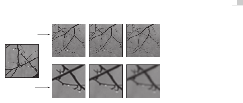
radius 1 radius 2 radius 3
Figure 9.39. The effects of using different sizes of a filter for upsampling (enlarging) or
downsampling (reducing) an image.
to handle the band of pixels within a filter radius of the edge (which require this
renormalization) separately from the center (which contains many more pixels
and does not require renormalization).
The choice of filter for resampling is important. There are two separate issues:
the shape of the filter and the size (radius). Because the filter serves both as a
reconstruction filter and a sampling filter, the requirements of both roles affect
the choice of filter. For reconstruction, we would like a filter smooth enough to
avoid aliasing artifacts when we enlarge the image, and the filter should be ripple-
free. For sampling, the filter should be large enough to avoid undersampling and
smooth enough to avoid moir´e artifacts. Figure 9.39 illustrates these two different
needs.
Generally we will choose one filter shape and scale it according to the relative
resolutions of the input and output. The lower of the two resolutions determines
the size of the filter: when the output is more coarsely sampled than the input
(downsampling, or shrinking the image), the smoothing required for proper sam-
pling is greater than the smoothing required for reconstruction, so we size the fil-
ter according to the output sample spacing (radius 3 in Figure 9.39). On the other
hand, when the output is more finely sampled (upsampling, or enlarging the im-
age) then the smoothing required for reconstruction dominates (the reconstructed
function is already smooth enough to sample at a higher rate than it started),
so the size of the filter is determined by the input sample spacing (radius 1 in
Figure 9.39).
Choosing the filter itself is a tradeoff between speed and quality. Common
choices are the box filter (when speed is paramount), the tent filter (moderate
quality), or a piecewise cubic (excellent quality). In the piecewise cubic case, the
i
i
i
i
i
i
i
i
218 9. Signal Processing
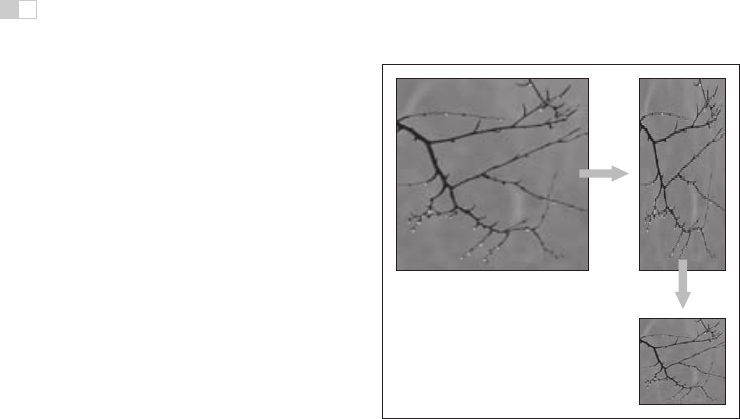
Figure 9.40. Resampling an image using a separable approach.
degree of smoothing can be adjusted by interpolating between f
B
and f
C
;the
Mitchell-Netravali filter is a good choice.
Just as with image filtering, separable filters can provide a significant speed-
up. The basic idea is to resample all the rows first, producing an image with
changed width but not height, then to resample the columns of that image to
produce the final result (Figure 9.40). Modifying the pseudocode given earlier so
that it takes advantage of this optimization is reasonably straightforward.
9.5 Sampling Theory
If you are only interested in implementation, you can stop reading here; the al-
gorithms and recommendations in the previous sections will let you implement
programs that perform sampling and reconstruction and achieve excellent results.
However, there is a deeper mathematical theory of sampling with a history reach-
ing back to the first uses of sampled representations in telecommunications. Sam-
pling theory answers many questions that are difficult to answer with reasoning
based strictly on scale arguments.
But most important, sampling theory gives valuable insight into the workings
of sampling and reconstruction. It gives the student who learns it an extra set of
intellectual tools for reasoning about how to achieve the best results with the most
efficient code.

i
i
i
i
i
i
i
i
9.5. Sampling Theory 219
n
πn
4
1
1
2
2
3
3
4
4
Figure 9.41. Approximating a square wave with finite sums of sines.
9.5.1 The Fourier Transform
The Fourier transform, along with convolution, is the main mathematical concept
that underlies sampling theory. You can read about the Fourier transform in many
math books on analysis, as well as in books on signal processing.
The basic idea behind the Fourier transform is to express any function by
adding together sine waves (sinusoids) of all frequencies. By using the appropri-
ate weights for the different frequencies, we can arrange for the sinusoids to add
up to any (reasonable) function we want.
As an example, the square wave in Figure 9.41 can be expressedby a sequence
of sine waves:
∞
n=1,3,5,...
4
πn
sin 2πnx.
This Fourier series starts with a sine wave (sin 2πx) that has frequency 1.0—same
as the square wave—and the remaining terms add smaller and smaller corrections
to reduce the ripples and, in the limit, reproduce the square wave exactly. Note
that all the terms in the sum have frequencies that are integer multiples of the
frequency of the square wave. This is because other frequencies would produce
results that don’t have the same period as the square wave.
A surprising fact is that a signal does not have to be periodic in order to be
expressed as a sum of sinusoids in this way: a non-periodic signal just requires
more sinusoids. Rather than summing over a discrete sequence of sinusoids, we
will instead integrate over a continuous family of sinusoids. For instance, a box
..................Content has been hidden....................
You can't read the all page of ebook, please click here login for view all page.