

i
i
i
i
i
i
i
i
220 9. Signal Processing
1
1
2
2
3
4
4
sin πu
πu
3
Figure 9.42. Approximating a box function with integrals of cosines up to each of four cutoff
frequencies.
function can be written as the integral of a family of cosine waves:
∞
−∞
sin πu
πu
cos 2πux du. (9.5)
This integral in Equation (9.5) is adding up infinitely many cosines, weighting
the cosine of frequency u by the weight (sin πu)/πu. The result, as we include
higher and higher frequencies, converges to the box function (see Figure 9.42).
When a function f is expressed in this way, this weight, which is a function of the
frequency u, is called the Fourier transform of f, denoted
ˆ
f. The function
ˆ
f tells
us how to build f by integrating over a family of sinusoids:
f(x)=
∞
−∞
ˆ
f(u)e
2πiux
du. (9.6)
Equation (9.6) is known as the inverse Fourier transform (IFT) because it starts
with the Fourier transform of f and ends up with f.
2
Note that in Equation (9.6) the complex exponential e
2πiux
has been substi-
tuted for the cosine in the previous equation. Also,
ˆ
f is a complex-valued func-
tion. The machinery of complex numbers is required to allow the phase, as well
2
Note that the term “Fourier transform” is used both for the function
ˆ
f and for the operation that
computes
ˆ
f from f . Unfortunately, this rather ambiguous usage is standard.

i
i
i
i
i
i
i
i
9.5. Sampling Theory 221
as the frequency, of the sinusoids to be controlled; this is necessary to represent
any functions that are not symmetric across zero. The magnitude of
ˆ
f is known
as the Fourier spectrum, and, for our purposes, this is sufficient—we won’t need
to worry about phase or use any complex numbers directly.
It turns out that computing
ˆ
f from f looks very much like computing f
from
ˆ
f:
ˆ
f(u)=
∞
−∞
f(x)e
−2πiux
dx. (9.7)
Equation (9.7) is known as the (forward) Fourier transform (FT). The sign in
the exponential is the only difference between the forward and inverse Fourier
transforms, and it is really just a technical detail. For our purposes, we can think
of the FT and IFT as the same operation.
Sometimes the f–
ˆ
f notation is inconvenient, and then we will denote the
Fourier transformof f by F{f }and the inverse Fourier transform of
ˆ
f by F
−1
{
ˆ
f}.
A function and its Fourier transform are related in many useful ways. A few
facts (most of them easy to verify) that we will use later in the chapter are:
• A function and its Fourier transform have the same squared integral:
x
f (x )
u
f (u )
̂
equal
energy
Figure 9.43. The Fourier
transform preserves the
squared integral of the
signal.
(f(x))
2
dx =
(
ˆ
f(u))
2
du.
The physical interpretation is that the two have the same energy (Figure
9.43).
In particular, scaling a function up by a also scales its Fourier transform by
a.Thatis,F{af} = aF{f}.
• Stretching a function along the x-axis squashes its Fourier transform along
the u-axis by the same factor (Figure 9.44):
F{f (x/b)} = b
ˆ
f(bx).
(The renormalization by b is needed to keep the energy the same.)
This means that if we are interested in a family of functions of different
width and height (say all box functions centered at zero), then we only
need to know the Fourier transform of one canonical function (say the box
function with width and height equal to one), and we can easily know the
Fourier transforms of all the scaled and dilated versions of that function.

i
i
i
i
i
i
i
i
222 9. Signal Processing
x
f (x )
x
f (x /2)
u
f (u )
̂
u
2f (2u )
̂
Figure 9.44. Scaling a signal along the
x
-axis in the space domain causes an inverse scale
along the
u
-axis in the frequency domain.
For example, we can instantly generalize Equation (9.5) to give the Fourier
transform of a box of width b and height a:
ab
sin πbu
πbu
.
• Theaveragevalueoff is equal to
ˆ
f(0). This makes sense since
ˆ
f(0) is sup-
posed to be the zero-frequency component of the signal (the DC component
if we are thinking of an electrical voltage).
• If f is real (which it always is for us),
ˆ
f is an even function—that is,
ˆ
f(u)=
ˆ
f(−u). Likewise, if f is an even function then
ˆ
f will be real (this is not
usually the case in our domain, but remember that we really are only going
to care about the magnitude of
ˆ
f).
9.5.2 Convolution and the Fourier Transform
One final property of the Fourier transform that deserves special mention is its
relationship to convolution (Figure 9.45). Briefly,
F{fg} =
ˆ
f ˆg.
i
i
i
i
i
i
i
i
9.5. Sampling Theory 223
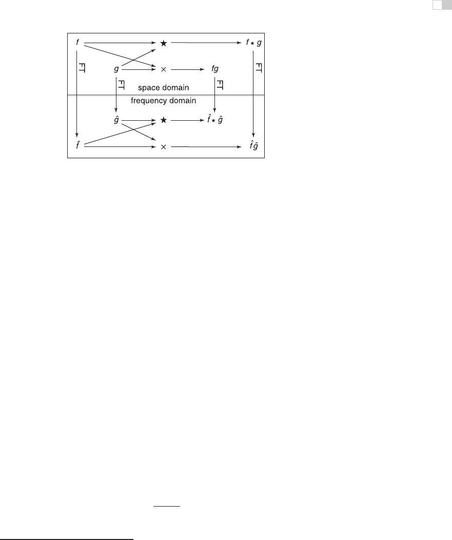
Figure 9.45. A commutative diagram to show visually the relationship between convolution
and multiplication. If we multiply
f
and
g
in space, then transform to frequency, we end up in
the same place as if we transformed
f
and
g
to frequency and then convolved them. Likewise,
if we convolve
f
and
g
in space and then transform into frequency, we end up in the same
place as if we transformed
f
and
g
to frequency, then multiplied them.
The Fourier transform of the convolution of two functions is the product of the
Fourier transforms. Following the by now familiar symmetry,
ˆ
fˆg = F{fg}.
The convolution of two Fourier transforms is the Fourier transform of the product
of the two functions. These facts are fairly straightforward to derive from the
definitions.
This relationship is the main reason Fourier transforms are useful in studying
the effects of sampling and reconstruction. We’ve seen how sampling, filtering,
and reconstruction can be seen in terms of convolution; now the Fourier transform
gives us a new domain—the frequency domain—in which these operations are
simply products.
9.5.3 A Gallery of Fourier Transforms
Now that we have some facts about Fourier transforms, let’s look at some exam-
ples of individual functions. In particular, we’ll look at some filters from Sec-
tion 9.3.1, which are shown with their Fourier transforms in Figure 9.46. We have
already seen the box function:
F{f
box
} =
sin πu
πu
= sinc πu.
The function
3
sin x/x is important enough to have its own name, sinc x.
3
You may notice that sin πu/πu is undefined for u =0. It is, however, continuous across zero,
and we take it as understood that we use the limiting value of this ratio, 1, at u =0.

i
i
i
i
i
i
i
i
224 9. Signal Processing
1
1
1
–1
1–1
x
u
f
tent
(x)
f
B
(x)
sinc
2
(u)
f
box
(x)sinc(u)
1
1
1
1–1
x
x
x u
–4 4
–4 4
u
u
sinc
4
(u)
1
–4 4
1
1–1
f
g
(x)
1
–4 4
2
3
1
√2π
√2π f
g
(2πu)
Figure 9.46. The Fourier transforms of the box, tent, B-spline, and Gaussian filters.
The tent function is the convolution of the box with itself, so its Fourier trans-
form is just the square of the Fourier transform of the box function:
F{f
tent
} =
sin
2
πu
π
2
u
2
=sinc
2
πu.
We can continue this process to get the Fourier transform of the B-spline filter
(see Exercise 3):
F{f
B
} =
sin
4
πu
π
4
u
4
=sinc
4
πu.
The Gaussian has a particularly nice Fourier transform:
F{f
G
} = e
−(2πu)
2
/2
.
It is another Gaussian! The Gaussian with standard deviation 1.0 becomes a Gaus-
sian with standard deviation 1/2π.
..................Content has been hidden....................
You can't read the all page of ebook, please click here login for view all page.