
i
i
i
i
i
i
i
i
286 12. Data Structures for Graphics
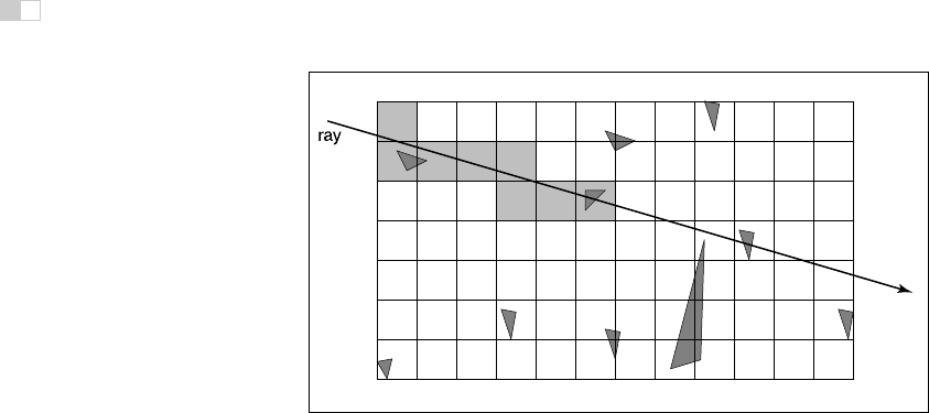
Figure 12.28. In uniform spatial subdivision, the ray is tracked forward through cells until
an object in one of those cells is hit. In this example, only objects in the shaded cells are
checked.
12.3.3 Uniform Spatial Subdivision
Another strategy to reduce intersection tests is to divide space. This is funda-
mentally different from dividing objects as was done with hierarchical bounding
volumes:
• In hierarchical bounding volumes, each object belongs to one of two sibling
nodes, whereas a point in space may be inside both sibling nodes.
• In spatial subdivision, each point in space belongs to exactly one node,
whereas objects may belong to many nodes.
In uniform spatial subdivision, the scene is partitioned into axis-aligned boxes.
These boxes are all the same size, although they are not necessarily cubes. The
ray traverses these boxes as shown in Figure 12.28. When an object is hit, the
traversal ends.
The grid itself should be a subclass of surface and should be implemented as
a 3D array of pointers to surface. For empty cells these pointers are NULL. For
cells with one object, the pointer points to that object. For cells with more than
one object, the pointer can point to a list, another grid, or another data structure,
such as a bounding volume hierarchy.
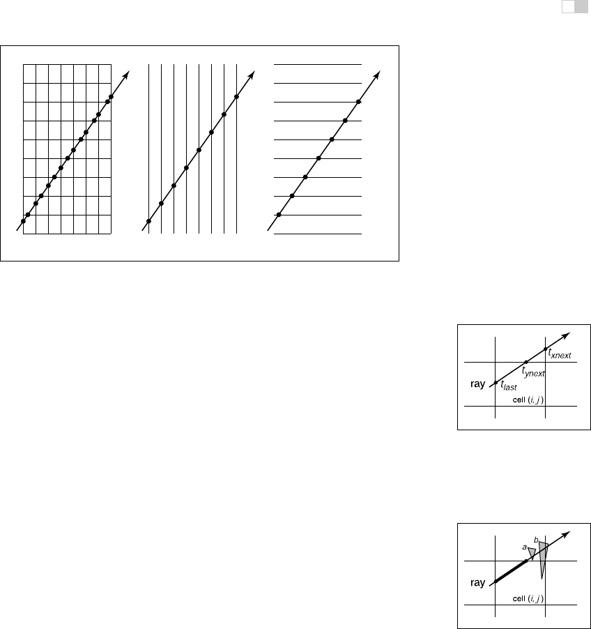
This traversal is done in an incremental fashion. The regularity comes from
the way that a ray hits each set of parallel planes, as shown in Figure 12.29. To
see how this traversal works, first consider the 2D case where the ray direction
has positive x and y components and starts outside the grid. Assume the grid is
bounded by points (x
min
,y
min
) and (x
max
,y
max
). The grid has n
x
× n
y
cells.
i
i
i
i
i
i
i
i
12.3. Spatial Data Structures 287
Figure 12.29. Although the pattern of cell hits seems irregular (left), the hits on sets of
parallel planes are very even.
Our first order of business is to find the index (i, j) of the first cell hit by
the ray e + td. Then, we need to traverse the cells in an appropriate order. The
key parts to this algorithm are finding the initial cell (i, j) and deciding whether
to increment i or j (Figure 12.30). Note that when we check for an intersection
Figure 12.30. To decide
whether we advance right
or upwards, we keep track
of the intersections with the
next vertical and horizontal
boundary of the cell.
with objects in a cell, we restrict the range of t to be within the cell (Figure 12.31).
Most implementations make the 3D array of type “pointer to surface.” To improve
the locality of the traversal, the array can be tiled as discussed in Section 12.5.
12.3.4 Axis-Aligned Binary Space Partitioning
Figure 12.31. Only hits
within the cell should be re-
ported. Otherwise the case
above would cause us to re-
port hitting object
b
rather
than object
a
.
We can also partition space in a hierarchical data structure such as a binary space
partitioning tree (BSP tree). This is similar to the BSP tree used for visibility
sorting in Section 12.4, but it’s most common to use axis-aligned, rather than
polygon-aligned, cutting planes for ray intersection.
A node in this structure contains a single cutting plane and a left and right
subtree. Each subtree contains all the objects on one side of the cutting plane.
Objects that pass through the plane are stored in in both subtrees. If we assume
the cutting plane is parallel to the yz plane at x = D, then the node class is:
class bsp-node subclass of surface
virtual bool hit(ray e + td, real t
0
, real t
1
, hit-record rec)
virtual box bounding-box()
surface-pointer left
surface-pointer right
real D
i
i
i
i
i
i
i
i
288 12. Data Structures for Graphics
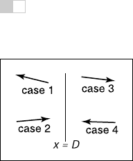
Figure 12.32. The four
cases of how a ray relates
to the BSP cutting plane
x=D
.
We generalize this to y and z cutting planes later. The intersection code can then
be called recursively in an object-oriented style. The code considers the four
cases shown in Figure 12.32. For our purposes, the origin of these rays is a point
at parameter t
0
:
p = a + t
0
b.
The four cases are:
1. The ray only interacts with the left subtree, and we need not test it for
intersection with the cutting plane. It occurs for x
p
<Dand x
b
< 0.
2. The ray is tested against the left subtree, and if there are no hits, it is then
tested against the right subtree. We need to find the ray parameter at x = D,
so we can make sure we only test for intersections within the subtree. This
case occurs for x
p
<Dand x
b
> 0.
3. This case is analogous to case 1 and occurs for x
p
>Dand x
b
> 0.
4. This case is analogous to case 2 and occurs for x
p
>Dand x
b
< 0.
The resulting traversal code handling these cases in order is:
function bool bsp-node::hit( ray a + tb, real t
0
, real t
1
, hit-record rec)
x
p
= x
a
+ t
0
x
b
if (x
p
<D) then
if (x
b
< 0) then
return (left = NULL) and (left→hit(a + tb, t
0
, t
1
,rec))
t =(D − x
a
)/x
b
if (t>t
1
) then
return (left = NULL) and (left→hit(a + tb, t
0
, t
1
,rec))
if (left = NULL) and (left→hit(a + tb, t
0
, t,rec)) then
return true
return (right = NULL) and (right→hit(a + tb, t, t
1
,rec))
else
analogous code for cases 3 and 4
This is very clean code. However, to get it started, we need to hit some root object
that includes a bounding box so we can initialize the traversal, t
0
and t
1
. An issue
we have to address is that the cutting plane may be along any axis. We can add
an integer index axis to the bsp-node class. If we allow an indexing operator
for points, this will result in some simple modifications to the code above, for
example,
i
i
i
i
i
i
i
i
12.4. BSP Trees for Visibility 289
x
p
= x
a
+ t
0
x
b
would become
u
p
= a[axis]+t
0
b[axis]
which will result in some additional array indexing, but will not generate more
branches.
While the processing of a single bsp-node is faster than processing a bvh-node,
the fact that a single surface may exist in more than one subtree means there are
more nodes and, potentially, a higher memory use. How “well” the trees are built
determines which is faster. Building the tree is similar to building the BVH tree.
We can pick axes to split in a cycle, and we can split in half each time, or we can
try to be more sophisticated in how we divide.
12.4 BSP Trees for Visibility
Another geometric problem in which spatial data structures can be used is deter-
mining the visibility ordering of objects in a scene with changing viewpoint.
If we are making many images of a fixed scene composed of planar polygons,
from different viewpoints—as is often the case for applications such as games—
we can use a binary space partitioning scheme closely related to the method for
ray intersection discussed in the previous section. The difference is that for vis-
ibility sorting we use non–axis-aligned splitting planes, so that the planes can be
made coincident with the polygons. This leads to an elegant algorithm known as
the BSP tree algorithm to order the surfaces from front to back. The key aspect
of the BSP tree is that it uses a preprocess to create a data structure that is useful
for any viewpoint. So, as the viewpoint changes, the same data structure is used
without change.
12.4.1 Overview of BSP Tree Algorithm
The BSP tree algorithm is an example of a painter’s algorithm. A painter’s algo-
rithm draws every object from back-to-front, with each new polygon potentially
overdrawing previous polygons, as is shown in Figure 12.33. It can be imple-
mented as follows:
sort objects back to front relative to viewpoint
for each object do
draw object on screen

i
i
i
i
i
i
i
i
290 12. Data Structures for Graphics
Figure 12.33. A painter’s algorithm starts with a blank image and then draws the scene one
object at a time from back-to-front, overdrawing whatever is already there. This automatically
eliminates hidden surfaces.
The problem with the first step (the sort) is that the relative order of multiple
objects is not always well defined, even if the order of every pair of objects is.
This problem is illustrated in Figure 12.34 where the three triangles form a cycle.
The BSP tree algorithm works on any scene composed of polygons where
no polygon crosses the plane defined by any other polygon. This restriction is
then relaxed by a preprocessing step. For the rest of this discussion, triangles are
assumed to be the only primitive, but the ideas extend to arbitrary polygons.
Figure 12.34. A cycle oc-
curs if a global back-to-front
ordering is not possible for
a particular eye position.
The basic idea of the BSP tree can be illustrated with two triangles, T
1
and
T
2
.Wefirst recall (see Section 2.5.3) the implicit plane equation of the plane
containing T
1
: f
1
(p)=0. The key property of implicit planes that we wish to
take advantage of is that for all points p
+
on one side of the plane, f
1
(p
+
) > 0;
..................Content has been hidden....................
You can't read the all page of ebook, please click here login for view all page.