
i
i
i
i
i
i
i
i
700 27. Visualization
With slicing, a single value is chosen from the dimension to eliminate, and
only the items matching that value for the dimension are extracted to include in
the lower-dimensional slice. Slicing is particularly useful with 3D spatial data, for
example when inspecting slices through a CT scan of a human head at different
heights along the skull. Slicing can be used to eliminate multiple dimensions at
once.
With projection, no information about the eliminated dimensions is retained;
the values for those dimensions are simply dropped, and all items are still shown.
A familiar form of projection is the standard graphics perspective transformation
which projects from 3D to 2D, losing information about depth along the way. In
mathematical visualization, the structure of higher-dimensional geometric objects
can be shown by projecting from 4D to 3D before the standard projection to the
image plane and using color to encode information from the projected-away di-
mension. This technique is sometimes called dimensional filtering when it is used
for nonspatial data.
In some datasets, there may be interesting hidden structure in a much lower-
dimensional space than the number of original data dimensions. For instance,
sometimes directly measuring the independent variables of interest is difficult or
impossible, but a large set of dependent or indirect variables is available. The goal
is to find a small set of dimensions that faithfully represent most of the structure or
variance in the dataset. These dimensions may be the original ones, or synthesized
new ones that are linear or nonlinear combinations of the originals. Principal com-
ponent analysis is a fast, widely used linear method. Many nonlinear approaches
have been proposed, including multidimensional scaling (MDS). These methods
are usually used to determine whether there are large-scale clusters in the dataset;
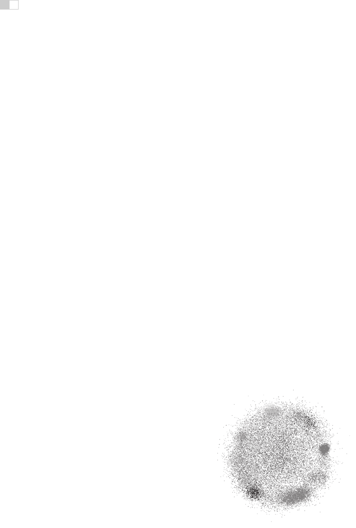
Figure 27.19. Dimensionality reduction with the Glimmer multidimensional scaling approach
shows clusters in a document dataset (Ingram et al., 2009),
c
2009 IEEE. (See also Plate L.)

i
i
i
i
i
i
i
i
27.8. Examples 701
the fine-grained structure in the lower-dimensional plots is usually not reliable
because information is lost in the reduction. Figure 27.19 shows document col-
lection in a single scatterplot. When the true dimensionality of the dataset is far
higher than two, a matrix of scatterplots showing pairs of synthetic dimensions
may be necessary.
27.8 Examples
We conclude this chapter with several examples of visualizing specific types of
data using the techniques discussed above.
27.8.1 Tables
Tabular data is extremely common, as all spreadsheet users know. The goal
in visualization is to encode this information through easily perceivable visual
channels rather than forcing people to read through it as numbers and text. Fig-
ure 27.20 shows the Table Lens, a focus+context approach where quantitative
Figure 27.20. The Table Lens provides focus+context interaction with tabular data, immedi-
ately reorderable by the values in each dimension column.
Image courtesy Stuart Card
(Rao
& Card, 1994),
c
1994 ACM, Inc. Included here by permission.

i
i
i
i
i
i
i
i
702 27. Visualization
Figure 27.21. Hierarchical parallel coordinates show high-dimensional data at multiple
levels of detail.
Image courtesy Matt Ward
(Fua et al., 1999),
c
1999 IEEE. (See also
Plate LI).
values are encoded as the length of one-pixel high lines in the context regions,
and shown as numbers in the focus regions. Each dimension of the dataset is
shown as a column, and the rows of items can be resorted according to the values
in that column with a single click in its header.
The traditional Cartesian approach of a scatterplot, where items are plotted
as dots with respect to perpendicular axes, is only usable for two and three di-
mensions of data. Many tables contain far more than three dimensions of data,
and the number of additional dimensions that can be encoded using other visual
channels is limited. Parallel coordinates are an approach for visualizing more di-
mensions at once using spatial position, where the axes are parallel rather than
perpendicular and an n-dimensional item is shown as a polyline that crosses each
of the n axes once (Inselberg & Dimsdale, 1990; Wegman, 1990). Figure 27.21
shows an 8-dimensional dataset of 230,000 items at multiple levels of detail (Fua
et al., 1999), from a high-level view at the top to finer detail at the bottom. With
hierarchical parallel coordinates, the items are clustered and an entire cluster of
items is represented by a band of varying width and opacity, where the mean is in
the middle and width at each axis depends on the values of the items in the cluster
in that dimension. The coloring of each band is based on the proximity between
clusters according to a similarity metric.
27.8.2 Graphs
The field of graph drawing is concerned with finding a spatial position for the
nodes in a graph in 2D or 3D space and routing the edges between these nodes
(Di Battista et al., 1999). In many cases the edge-routing problem is simpli-

i
i
i
i
i
i
i
i
27.8. Examples 703
fied by using only straight edges, or by only allowing right-angle bends for the
class of orthogonal layouts, but some approaches handle true curves. If the graph
has directed edges, a layered approach can be used to show hierarchical struc-
ture through the horizontal or vertical spatial ordering of nodes, as shown in Fig-
ure 27.2.
Figure 27.22. Graph lay-
out aesthetic criteria. Top:
Edge crossings should be
minimized. Middle: Angular
resolution should be max-
imized. Bottom: Symme-
try is maximized on the left,
whereas crossings are min-
imized on the right, showing
the conflict between the in-
dividually NP-hard criteria.
A suite of aesthetic criteria operationalize human judgements about readable
graphs as metrics that can be computed on a proposed layout (Ware et al., 2002).
Figure 27.22 shows some examples. Some metrics should be minimized, such
as the number of edge crossings, the total area of the layout, and the number of
right-angle bends or curves. Others should be maximized, such as the angular
resolution or symmetry. The problem is difficult because most of these criteria
are individually NP-hard, and moreover they are mutually incompatible (Bran-
denburg, 1988).
Many approaches to node-link graph drawing use force-directed placement,
motivated by the intuitive physical metaphor of spring forces at the edges drawing
together repelling particles at the nodes. Although naive approaches have high
time complexity and are prone to being caught in local minima, much work has
gone into developing more sophisticated algorithms such as GEM (Frick et al.,
1994) or IPSep-CoLa (Dwyer et al., 2006). Figure 27.23 shows an interactive
system using the r-PolyLog energy model, where a focus+context view of the
clustered graph is created with both geometric and semantic fisheye (van Ham &
van Wijk, 2004).
Figure 27.23. Force-directed placement showing a clustered graph with both geometric
and semantic fisheye.
Image courtesy Jarke van Wijk
(van Ham & van Wijk, 2004),
c
2004
IEEE.

i
i
i
i
i
i
i
i
704 27. Visualization
Figure 27.24. Graphs can be shown with either matrix or node-link views.
Image courtesy
Jean-Daniel Fekete
(Henry & Fekete, 2006),
c
2006 IEEE.
Graphs can also be visually encoded by showing the adjacency matrix, where
all vertices are placed along each axis and the cell between two vertices is colored
if there is an edge between them. The MatrixExplorer system uses linked multi-
ple views to help social science researchers visually analyze social networks with
both matrix and node-link representations (Henry & Fekete, 2006). Figure 27.24
shows the different visual patterns created by the same graph structure in these
two views: A represents an actor connecting several communities; B is a com-
munity; and C is a clique, or a complete sub-graph. Matrix views do not suffer
from cluttered edge crossings, but many tasks including path following are more
difficult with this approach.
27.8.3 Trees
Trees are a special case of graphs so common that a great deal of visualization
research has been devoted to them. A straightforward algorithm to lay out trees in
the two-dimensional plane works well for small trees (Reingold & Tilford, 1981),
while a more complex but scalable approach runs in linear time (Buchheim et
al., 2002). Figures 27.17 and 27.18 also show trees with different approaches
to spatial layout, but all four of these methods visually encode the relationship
between parent and child nodes by drawing a link connecting them.
..................Content has been hidden....................
You can't read the all page of ebook, please click here login for view all page.