

i
i
i
i
i
i
i
i
4.4. Ray-Object Intersection 79
t =
x
a
− x
b
x
a
− x
c
x
a
− x
e
y
a
− y
b
y
a
− y
c
y
a
− y
e
z
a
− z
b
z
a
− z
c
z
a
− z
e
|A|
,
where the matrix A is
A =
⎡
⎣
x
a
− x
b
x
a
− x
c
x
d
y
a
− y
b
y
a
− y
c
y
d
z
a
− z
b
z
a
− z
c
z
d
⎤
⎦
,
and |A| denotes the determinant of A.The3 ×3 determinants have common sub-
terms that can be exploited. Looking at the linear systems with dummy variables
⎡
⎣
adg
beh
cf i
⎤
⎦
⎡
⎣
β
γ
t
⎤
⎦
=
⎡
⎣
j
k
l
⎤
⎦
,
Cramer’s rule gives us
β =
j(ei − hf )+k(gf − di)+l(dh − eg)
M
,
γ =
i(ak −jb)+h(jc −al)+g(bl − kc)
M
,
t = −
f(ak − jb)+e(jc − al)+d(bl − kc)
M
,
where
M = a(ei − hf )+b(gf − di)+c(dh − eg).
We can reduce the number of operations by reusing numbers such as
“ei-minus-hf.”
The algorithm for the ray-triangle intersection for which we need the linear so-
lution can have some conditions for early termination. Thus, the function should
look something like:
boolean raytri (ray r, vector3 a, vector3 b, vector3 c,interval[t
0
,t
1
])
compute t
if (t<t
0
) or (t>t
1
) then
return false
compute γ
if (γ<0) or (γ>1) then
return false

i
i
i
i
i
i
i
i
80 4. Ray Tracing
compute β
if (β<0) or (β>1 − γ) then
return false
return true
4.4.3 Ray-Polygon Intersection
Given a planar polygon with m vertices p
1
through p
m
and surface normal n,
we first compute the intersection points between the ray e + td and the plane
containing the polygon with implicit equation
(p − p
1
) · n =0.
We do this by setting p = e + td and solving for t to get
t =
(p
1
− e) · n
d · n
.
This allows us to compute p.Ifp is inside the polygon, then the ray hits it, and
otherwise it does not.
We can answer the question of whether p is inside the polygon by projecting
the point and polygon vertices to the xy plane and answering it there. The easiest
waytodothisistosendany2Drayoutfromp and to count the number of
intersections between that ray and the boundary of the polygon (Sutherland et al.,
1974; Glassner, 1989). If the number of intersections is odd, then the point is
inside the polygon; otherwise it is not. This is true because a ray that goes in
must go out, thus creating a pair of intersections. Only a ray that starts inside
will not create such a pair. To make computation simple, the 2D ray may as well
propagate along the x-axis:
x
y
=
x
p
y
p
+ s
1
0
.
It is straightforward to compute the intersection of that ray with the edges such as
(x
1
,y
1
,x
2
,y
2
) for s ∈ (0, ∞).
A problem arises, however, for polygons whose projection into the xy plane
is a line. To get around this, we can choose among the xy, yz,orzx planes for
whichever is best. If we implement our points to allow an indexing operation,
e.g., p(0) = x
p
then this can be accomplished as follows:
if (abs(z
n
) > abs(x
n
)) and (abs(z
n
) > abs(y
n
)) then
index0 = 0

i
i
i
i
i
i
i
i
4.5. Shading 81
index1 = 1
else if (abs(y
n
) > abs (x
n
)) then
index0 = 0
index1 = 2
else
index0 = 1
index1 = 2
Now, all computations can use p(index0) rather than x
p
, and so on.
Another approach to polygons, one that is often used in practice, is to replace
them by several triangles.
4.4.4 Intersecting a Group of Objects
Of course, most interesting scenes consist of more than one object, and when we
intersect a ray with the scene we must find only the closest intersection to the
camera along the ray. A simple way to implement this is to think of a group of
objects as itself being another type of object. To intersect a ray with a group, you
simply intersect the ray with the objects in the group and return the intersection
with the smallest t value. The following code tests for hits in the interval t ∈
[t
0
,t
1
]:
Figure 4.11. Asimple
scene rendered with only
ray generation and surface
intersection, but no shad-
ing; each pixel is just set to
a fixed color depending on
which object it hit.
hit = false
for each object o in the group do
if (o ishitatrayparametert and t ∈ [t
0
,t
1
]) then
hit = true
hitobject = o
t
1
= t
return hit
4.5 Shading
Once the visible surface for a pixel is known, the pixel value is computed by eval-
uating a shading model. How this is done depends entirely on the application—
methods range from very simple heuristics to elaborate numerical computations.
In this chapter we describe the two most basic shading models; more advanced
models are discussed in Chapter 10.
Most shading models, one way or another, are designed to capture the process
of light reflection, whereby surfaces are illuminated by light sources and reflect

i
i
i
i
i
i
i
i
82 4. Ray Tracing
part of the light to the camera. Simple shading models are defined in terms of
illumination from a point light source. The important variables in light reflection
are the light direction l, which is a unit vector pointing towards the light source;
the view direction v, which is a unit vector pointing toward the eye or camera; the
surface normal n, which is a unit vector perpendicular to the surface at the point
where reflection is taking place; and the characteristics of the surface—color,
shininess, or other properties depending on the particular model.
4.5.1 Lambertian Shading
Illumination from real point
sources falls off as distance
squared, but that is often
more trouble than it’s worth
in a simple renderer.
The simplest shading model is based on an observation made by Lambert in the
18th century: the amount of energy from a light source that falls on an area of
surface depends on the angle of the surface to the light. A surface facing directly
towards the light receives maximum illumination; a surface tangent to the light
direction (or facing away from the light) receives no illumination; and in between
the illumination is proportional to the cosine of the angle θ between the surface
normal and the light source (Figure 4.12). This leads to the Lambertian shading
model:
L = k
d
I max(0, n · l)
where L is the pixel color; k
d
is the diffuse coefficient, or the surface color; and
I is the intensity of the light source. Because n and l are unit vectors, we can
l
n
v
Figure 4.12. Geometry for
Lambertian shading.
use n · l as a convenient shorthand (both on paper and in code) for cos θ.This
equation (as with the other shading equations in this section) applies separately to
the three color channels, so the red component of the pixel value is the product of
the red diffuse component, the red light source intensity, and the dot product; the
same holds for green and blue.
When in doubt, make light
sources neutral in color,
with equal red, green, and
blue intensities.
The vector l is computed by subtracting the intersection point of the ray and
surface from the light source position. Don’t forget that v, l,andn all must be
unit vectors; failing to normalize these vectors is a very common error in shading
computations.
4.5.2 Blinn-Phong Shading
Lambertian shading is view independent: the color of a surface does not depend
on the direction from which you look. Many real surfaces show some degree
of shininess, producing highlights, or specular reflections, that appear to move
around as the viewpoint changes. Lambertian shading doesn’t produce any high-
lights and leads to a very matte, chalky appearance, and many shading models
i
i
i
i
i
i
i
i
4.5. Shading 83
Figure 4.13. Asimple
scene rendered with diffuse
shading from a single light
source.
Figure 4.14. Asimple
scene rendered with diffuse
shading and shadows (Sec-
tion 4.7) from three light
sources.
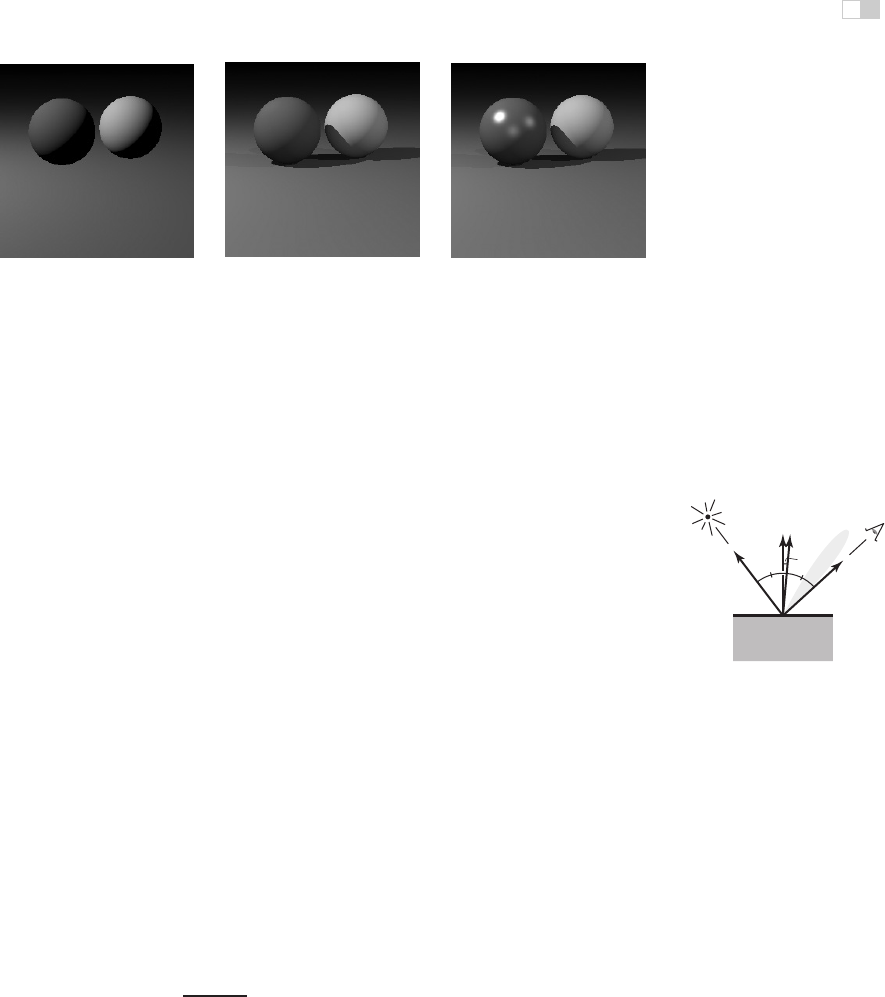
Figure 4.15. Asim-
ple scene rendered with dif-
fuse shading (right), Blinn-
Phong shading (left), and
shadows (Section 4.7) from
three light sources.
add a specular component to Lambertian shading; the Lambertian part is then the
diffuse component.
A very simple and widely used model for specular highlights was proposed
by Phong (Phong, 1975) and later updated by Blinn (J. F. Blinn, 1976) to the form
most commonly used today. The idea is to produce reflection that is at its brightest
when v and l are symmetrically positioned across the surface normal, which is
when mirror reflection would occur; the refelction then decreases smoothly as the
vectors move away from a mirror configuration.
l
n
h
v
Figure 4.16. Geometry for
Blinn-Phong shading.
We can tell how close we are to a mirror configuration by comparing the
half vector h (the bisector of the angle between v and l) to the surface normal
(Figure 4.16). If the half vector is near the surface normal, the specular component
should be bright; if it is far away it should be dim. This result is achieved by
computing the dot product between h and n (remember they are unit vectors, so
Typical values of
p
: 10—
“eggshell”; 100—mildly
shiny; 1000—really glossy;
10,000—nearly mirror-like.
n ·h reaches its maximum of 1 when the vectors are equal), then taking the result
to a power p>1 to make it decrease faster. The power, or Phong exponent,
controls the apparent shininess of the surface. The half vector itself is easy to
compute: since v and l are the same length, their sum is a vector that bisects the
angle between them, which only needs to be normalized to produce h.
Putting this all together, the Blinn-Phong shading model is as follows:
When in doubt, make the
specular color gray, with
equal red, green, and blue
values.
h =
v + l
v + l
,
L = k
d
I max(0, n · l)+k
s
I max(0, n ·h)
p
,
where k
s
is the specular coefficient, or the specular color, of the surface.
..................Content has been hidden....................
You can't read the all page of ebook, please click here login for view all page.