
i
i
i
i
i
i
i
i
9.3. Convolution Filters 205
the samples when used as a reconstruction filter (Section 9.3.2):
f
C
(x)=
1
2
⎧
⎪
⎨
⎪
⎩
−3(1 −|x|)
3
+4(1−|x|)
2
+(1−|x|) −1 ≤ x ≤ 1,
(2 −|x|)
3
− (2 −|x|)
2
1 ≤|x|≤2,
0 otherwise.
The Mitchell-Netravali Cubic Filter
For the all-important application of resampling images, Mitchell and Netravali
(Mitchell & Netravali, 1988) made a study of cubic filters and recommended one
part way between the previous two filters as the best all-around choice (Figure
9.24). It is simply a weighted combination of the previous two filters:
8
9
1
1
2–1–2
x
Figure 9.24. The Mitchell-
Netravali filter.
f
M
(x)=
1
3
f
B
(x)+
2
3
f
C
(x)
=
1
18
⎧
⎪
⎨
⎪
⎩
−21(1 −|x|)
3
+ 27(1 −|x|)
2
+9(1−|x|)+1 −1 ≤ x ≤ 1,
7(2 −|x|)
3
− 6(2 −|x|)
2
1 ≤|x|≤2,
0 otherwise.
9.3.2 Properties of Filters
Filters have some traditional terminology that goes with them, which we use to
describe the filters and compare them to one another.
The impulse response of a filter is just another name for the function: it is
the response of the filter to a signal that just contains an impluse (and recall that
convolving with an impulse just gives back the filter).
0 0 1 0 0
reconstructed
signal
samples
filter
weights
Figure 9.25. An interpolating filter reconstructs
the sample points exactly because it has the
value zero at all non-zero integer offsets from
the center.
A continuous filter is interpolat-
ing if, when it is used to reconstruct
a continuous function from a dis-
crete sequence, the resulting func-
tion takes on exactly the values of
the samples at the sample points—
that is, it “connects the dots” rather
than producing a function that only
goes near the dots. Interpolating fil-
ters are exactly those filters f for
which f(0) = 1 and f(i)=0for all non-zero integers i (Figure 9.25).

i
i
i
i
i
i
i
i
206 9. Signal Processing
overshoot
overshoot
Figure 9.26. A filter with negative lobes will
always produce some overshoot when filtering
or reconstructing a sharp discontinuity.
A filter that takes on negative
values has ringing or overshoot:it
will produce extra oscillations in the
value around sharp changes in the
value of the function being filtered.
For instance, the Catmull-Rom
filter has negative lobes on either
side, and if you filter a step function
with it, it will exaggerate the step a bit, resulting in function values that under-
shoot 0 and overshoot 1 (Figure 9.26).
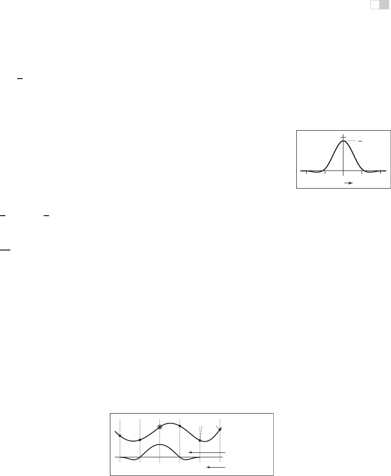
A continuous filter is ripple free if, when used as a reconstruction filter, it
will reconstruct a constant sequence as a constant function (Figure 9.27). This is
equivalent to the requirement that the filter sum to one on any integer-spaced grid:
i
f(x + i)=1 for all x.
A continuous filter has a degree of continuity, which is the highest-order
derivative that is defined everywhere. A filter, like the box filter, that has sud-
den jumps in its value is not continuous at all. A filter that is continuous but
has sharp corners (discontinuities in the first derivative), such as the tent filter,
has order of continuity zero, and we say it is C
0
.Afilter that has a continuous
derivative (no sharp corners), such as the piecewise cubic filters in the previous
section, is C
1
; if its second derivative is also continuous, as is true of the B-spline
filter, it is C
2
. The order of continuity of a filter is particularly important for a
reconstruction filter because the reconstructed function inherits the continuity of
the filter.
ripple-free
not ripple-free
Σ = 1
Σ ≠ 1
Figure 9.27. The tent filter of radius 1 is a ripple-free reconstruction filter; the Gaussian
filter with standard deviation 1/2 is not.
i
i
i
i
i
i
i
i
9.3. Convolution Filters 207
Separable Filters
So far we have only discussed filters for 1D convolution, but for images and other
multidimensional signals we need filters too. In general, any 2D function could
bea2Dfilter, and occasionally it is useful to define them this way. But, in most
cases, we can build suitable 2D (or higher-dimensional) filters from the 1D filters
we have already seen.
The most useful way of doing this is by using a separable filter. The value of
a separable filter f
2
(x, y) at a particular x and y is simply the product of f
1
(the
1D filter) evaluated at x and at y:
f
2
(x, y)=f
1
(x)f
1
(y).
Similarly, for discrete filters,
a
2
[i, j]=a
1
[i]a
1
[j].
Any horizontal or vertical slice through f
2
is a scaled copy of f
1
. The integral of
f
2
is the square of the integral of f
1
, so in particular if f
1
is normalized, then so
is f
2
.
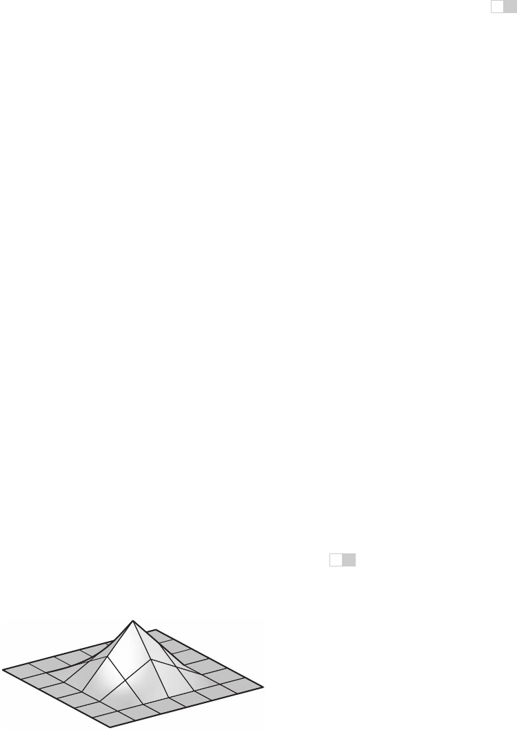
Example (The separable tent filter). If we choose the tent function for f
1
,there-
sulting piecewise bilinear function (Figure 9.28) is
f
2,tent
(x, y)=
(1 −|x|)(1 −|y|) |x| < 1 and |y| < 1,
0 otherwise.
The profiles along the coordinate axes are tent functions, but the profiles along
the diagonals are quadratics (for instance, along the line x = y in the positive
quadrant, we see the quadratic function (1 − x)
2
).
Figure 9.28. The separable 2D tent filter.
i
i
i
i
i
i
i
i
208 9. Signal Processing
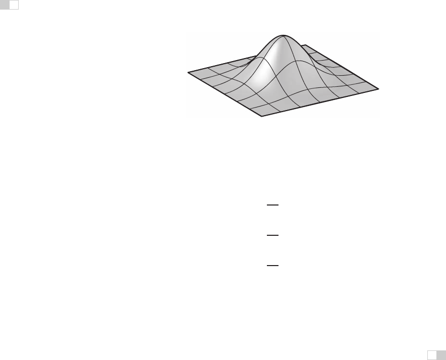
Figure 9.29. The 2D Gaussian filter, which is both separable and radially symmetric.
Example (The 2D Gaussian filter). If we choose the Gaussian function for f
1
,the
resulting 2D function (Figure 9.29) is
f
2,g
(x, y)=
1
2π
e
−x
2
/2
e
−y
2
/2
,
=
1
2π
e
−(x
2
+y
2
)/2
,
=
1
2π
e
−r
2
/2
.
Notice that this is (up to a scale factor) the same function we would get if we
revolved the 1D Gaussian around the origin to produce a circularly symmetric
function. The property of being both circularly symmetric and separable at the
same time is unique to the Gaussian function. The profiles along the coordinate
axes are Gaussians, but so are the profiles along any direction at any offset from
the center.
The key advantage of separable filters over other 2D filters has to do with ef-
ficiency in implementation. Let’s substitute the definition of a
2
into the definition
of discrete convolution:
(a
2
b)[i, j]=
i
j
a
1
[i
]a
1
[j
]b[i − i
,j− j
].
Note that a
1
[i
] does not depend on j
and can be factored out of the inner sum:
=
i
a
1
[i
]
j
a
1
[j
]b[i − i
,j− j
].
i
i
i
i
i
i
i
i
9.3. Convolution Filters 209
Let’s abbreviate the inner sum as S[k]:
S[k]=
j
a
1
[j
]b[k, j − j
];
(a
2
b)[i, j]=
i
a
1
[i
]S[i − i
]. (9.4)
With the equation in this form, we can first compute and store S[i − i
] for each
value of i
, and then compute the outer sum using these stored values. At first
glance this does not seem remarkable, since we still had to do work proportional
to (2r +1)
2
to compute all the inner sums. However, it’s quite different if we
want to compute the value at many points [i, j].
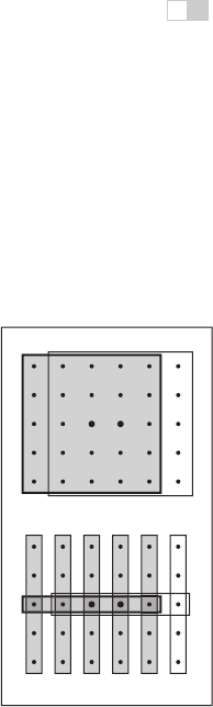
Suppose we need to compute a
2
bat [2, 2] and [3, 2],anda
1
has a radius
of 2. Examining Equation (9.4), we can see that we will need S[0],...,S[4] to
compute the result at [2, 2], and we will need S[1],...,S[5] to compute the result
at [3, 2]. So, in the separable formulation, we can just compute all six values of S
and share S[1],...,S[4] (Figure 9.30).
This savings has great significance for large filters. Filtering an m by n 2D
image with a filter of radius r in the general case requires computationof (2r+1)
2
products per pixel, while filtering the image with a separable filterofthesamesize
requires 2(2r +1)products (at the expense of some intermediate storage). This
change in asymptotic complexity from O(r
2
) to O(r) enables the use of much
larger filters.
Figure 9.30. Com-
puting two output points
using separate 2D arrays
of 25 samples (above) vs.
filtering once along the
columns, then using sepa-
rate 1D arrays of five sam-
ples (below).
The algorithm is:
function filterImage(image I, filter f)
r = f.radius
n
x
= I.width
n
y
= I.height
allocate storage array S[0,...,n
x
− 1]
allocate image I
out
[r,...,n
x
− r − 1][r,...,n
y
− r − 1]
initialize S and I
out
to all zero
for y = r to n
y
− r − 1 do
for x =0to n
x
− 1 do
S[x]=0
for i = −r to r do
S[x]=S[x]+f[i]I[x][y −i]
for x = r to n
x
− r − 1 do
for i = −r to r do
I
out
[x][y]=I
out
[x][y]+f[i]S[x − i]
return I
out
..................Content has been hidden....................
You can't read the all page of ebook, please click here login for view all page.