

i
i
i
i
i
i
i
i
146 7. Viewing
To draw 3D line segments in the orthographic view volume, we project them
into screen x-andy-coordinates and ignore z-coordinates. We do this by com-
bining Equations (7.2) and (7.3). Note that in a program we multiply the matrices
together to form one matrix and then manipulate points as follows:
⎡
⎢
⎢
⎣
x
pixel
y
pixel
z
canonical
1
⎤
⎥
⎥
⎦
=(M
vp
M
orth
)
⎡
⎢
⎢
⎣
x
y
z
1
⎤
⎥
⎥
⎦
.
The z-coordinate will now be in [−1, 1]. We don’t take advantage of this now, but
it will be useful when we examine z-buffer algorithms.
The code to draw many 3D lines with endpoints a
i
and b
i
thus becomes both
simple and efficient:
This is a first example of
how matrix transformation
machinery makes graphics
programs clean and effi-
cient.
construct M
vp
construct M
orth
M = M
vp
M
orth
for each line segment (a
i
, b
i
) do
p = Ma
i
q = Mb
i
drawline(x
p
,y
p
,x
q
,y
q
)
7.1.3 The Camera Transformation
We’d like to able to change the viewpoint in 3D and look in any direction. There
are a multitude of conventions for specifying viewer position and orientation. We
will use the following one (see Figure 7.6):
Figure 7.6. The user
specifies viewing as an eye
position e, a gaze direc-
tion g, and an up vector
t. We construct a right-
handed basis with w point-
ing opposite to the gaze
and v being in the same
plane as g and t.
• the eye position e,
• the gaze direction g ,
• the view-up vector t.
The eye position is a location that the eye “sees from.” If you think of graphics
as a photographic process, it is the center of the lens. The gaze direction is any
vector in the direction that the viewer is looking. The view-up vector is any vector
in the plane that both bisects the viewer’s head into right and left halves and points
“to the sky” for a person standing on the ground. These vectors provide us with
enough information to set up a coordinate system with origin e and a uvw basis,

i
i
i
i
i
i
i
i
7.1. Viewing Transformations 147
Figure 7.7. For arbitrary viewing, we need to change the points to be stored in the “appro-
priate” coordinate system. In this case it has origin e and offset coordinates in terms of uvw.
using the construction of Section 2.4.7:
w = −
g
g
,
u =
t × w
t × w
,
v = w × u.
Our job would be done if all points we wished to transform were stored in co-
ordinates with origin e and basis vectors u, v,andw. But as shown in Figure 7.7,
the coordinates of the model are stored in terms of the canonical (or world) ori-
gin o and the x-, y-, and z-axes. To use the machinery we have already developed,
we just need to convert the coordinates of the line segment endpoints we wish to
draw from xyz-coordinates into uvw-coordinates. This kind of transformation
was discussed in Section 6.5, and the matrix that enacts this transformation is the
canonical-to-basis matrix of the camera’s coordinate frame:
M
cam
=
uvwe
0001
−1
=
⎡
⎢
⎢
⎣
x
u
y
u
z
u
0
x
v
y
v
z
v
0
x
w
y
w
z
w
0
0001
⎤
⎥
⎥
⎦
⎡
⎢
⎢
⎣
100−x
e
010−y
e
001−z
e
000 1
⎤
⎥
⎥
⎦
. (7.4)
Alternatively, we can think of this same transformation as first moving e to the
origin, then aligning u, v, w to x, y, z.
To make our previously z-axis-only viewing algorithm work for cameras with
any location and orientation, we just need to add this camera transformation
i
i
i
i
i
i
i
i
148 7. Viewing
to the product of the viewport and projection transformations, so that it con-
verts the incoming points from world to camera coordinates before they are pro-
jected:
construct M
vp
construct M
orth
construct M
cam
M = M
vp
M
orth
M
cam
for each line segment (a
i
, b
i
) do
p = Ma
i
q = Mb
i
drawline(x
p
,y
p
,x
q
,y
q
)
Again, almost no code is needed once the matrix infrastructure is in place.
7.2 Projective Transformations
We have left perspective for last because it takes a little bit of cleverness to make
it fit into the system of vectors and matrix transformations that has served us so
well up to now. To see what we need to do, let’s look at what the perspective
projection transformation needs to do with points in camera space. Recall that the
For the moment we will ig-
nore the sign of
z
to keep
the equations simpler, but it
will return on page 152.
viewpoint is positioned at the origin and the camera is looking along the z-axis.
The key property of perspective is that the size of an object on the screen is
proportional to 1/z for an eye at the origin looking up the negative z-axis. This
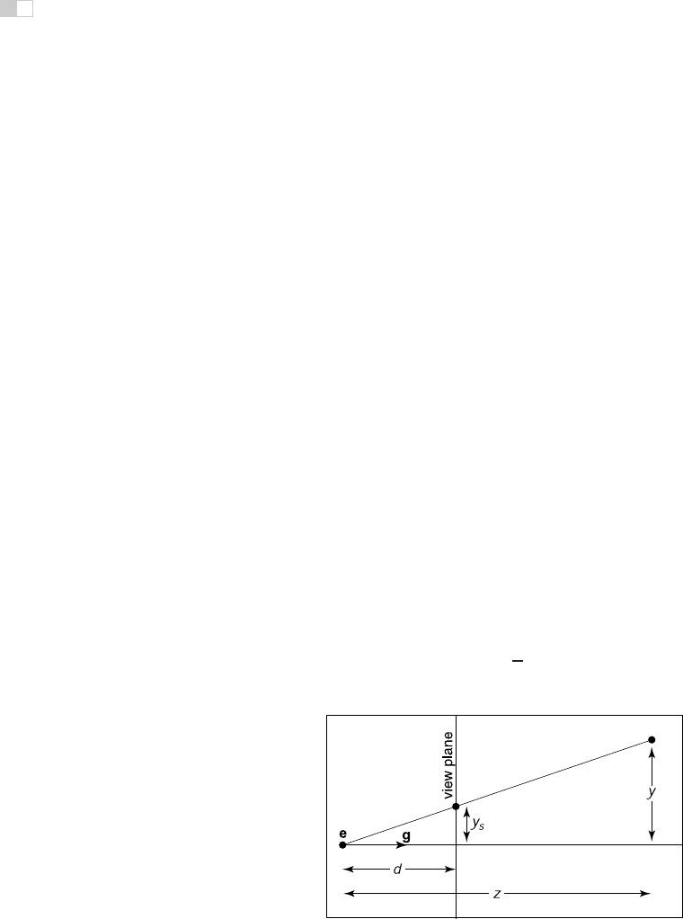
can be expressed more precisely in an equation for the geometry in Figure 7.8:
y
s
=
d
z
y, (7.5)
Figure 7.8. The geometry for Equation (7.5). The viewer’s eye is at e and the gaze direction
is g (the minus
z
-axis). The view plane is a distance
d
from the eye. A point is projected
toward e and where it intersects the view plane is where it is drawn.

i
i
i
i
i
i
i
i
7.2. Projective Transformations 149
where y is the distance of the point along the y-axis, and y
s
is where the point
should be drawn on the screen.
We would really like to use the matrix machinery we developed for ortho-
graphic projection to draw perspective images; we could then just multiply an-
other matrix into our composite matrix and use the algorithm we already have.
However, this type of transformation, in which one of the coordinates of the input
vector appears in the denominator, can’t be achieved using affine transformations.
We can allow for division with a simple generalization of the mechanism of
homogeneous coordinates that we have been using for affine transformations.
We have agreed to represent the point (x, y, z) using the homogeneous vector
[xyz1]
T
; the extra coordinate, w,isalwaysequalto1, and this is ensured by
always using [0001]
T
as the fourth row of an affine transformation matrix.
Rather than just thinking of the 1 as an extra piece bolted on to coerce matrix
multiplication to implement translation, we now define it to be the denominator
of the x-, y-, and z-coordinates: the homogeneous vector [xyzw]
T
represents
the point (x/w, y/w, z/w). This makes no difference when w =1, but it allows a
broader range of transformations to be implemented if we allow any values in the
bottom row of a transformation matrix, causing w to take on values other than 1.
Concretely, linear transformations allow us to compute expressions like
x
= ax + by + cz
and affine transformations extend this to
x
= ax + by + cz + d.
Treating w as the denominator further expands the possibilities, allowing us to
compute functions like
x
=
ax + by + cz + d
ex + fy + gz + h
;
this could be called a “linear rational function” of x, y,andz. But there is an extra
constraint—the denominators are the same for all coordinates of the transformed
point:
x
=
a
1
x + b
1
y + c
1
z + d
1
ex + fy + gz + h
,
y
=
a
2
x + b
2
y + c
2
z + d
2
ex + fy + gz + h
,
z
=
a
3
x + b
3
y + c
3
z + d
3
ex + fy + gz + h
.

i
i
i
i
i
i
i
i
150 7. Viewing
Expressed as a matrix transformation,
⎡
⎢
⎢
⎣
˜x
˜y
˜z
˜w
⎤
⎥
⎥
⎦
=
⎡
⎢
⎢
⎣
a
1
b
1
c
1
d
1
a
2
b
2
c
2
d
2
a
3
b
3
c
3
d
3
efgh
⎤
⎥
⎥
⎦
⎡
⎢
⎢
⎣
x
y
z
1
⎤
⎥
⎥
⎦
and
(x
,y
,z
)=(˜x/ ˜w, ˜y/ ˜w, ˜z/ ˜w).
A transformation like this is known as a projective transformation or a
homography.
Example. The matrix
M =
⎡
⎣
20−1
03 0
0
2
3
1
3
⎤
⎦
represents a 2D projective transformation that transforms the unit square ([0, 1] ×
[0, 1]) to the quadrilateral shown in Figure 7.9.
1
1
3
3
1
unit
square
Figure 7.9. Aprojec-
tive transformation maps a
square to a quadrilateral,
preserving straight lines but
not parallel lines.
For instance, the lower-right corner of the square at (1, 0) is represented by
the homogeneous vector [1 0 1]
T
and transforms as follows:
⎡
⎣
20−1
03 0
0
2
3
1
3
⎤
⎦
⎡
⎣
1
0
1
⎤
⎦
=
⎡
⎣
1
0
1
3
⎤
⎦
,
which represents the point (1/
1
3
, 0/
1
3
),or(3, 0).Notethatifweusethematrix
3M =
⎡
⎣
60−3
09 0
02 1
⎤
⎦
instead, the result is [301]
T
, which also represents (3, 0). In fact, any scalar
multiple cM is equivalent: the numerator and denominator are both scaled by c,
which does not change the result.
There is a more elegant way of expressingthe same idea, which avoids treating
the w-coordinate specially. In this view a 3D projective transformation is simply
a 4D linear transformation, with the extra stipulation that all scalar multiples of a
vector refer to the same point:
x ∼ αx for all α =0.
The symbol ∼ is read as “is equivalent to” and means that the two homogeneous
vectors both describe the same point in space.
..................Content has been hidden....................
You can't read the all page of ebook, please click here login for view all page.