
i
i
i
i
i
i
i
i
5
Linear Algebra
Perhaps the most universal tools of graphics programs are the matrices that
change or transform points and vectors. In the next chapter, we will see
how a vector can be represented as a matrix with a single column, and how
the vector can be represented in a different basis via multiplication with a
square matrix. We will also describe how we can use such multiplications to
accomplish changes in the vector such as scaling, rotation, and translation. In this
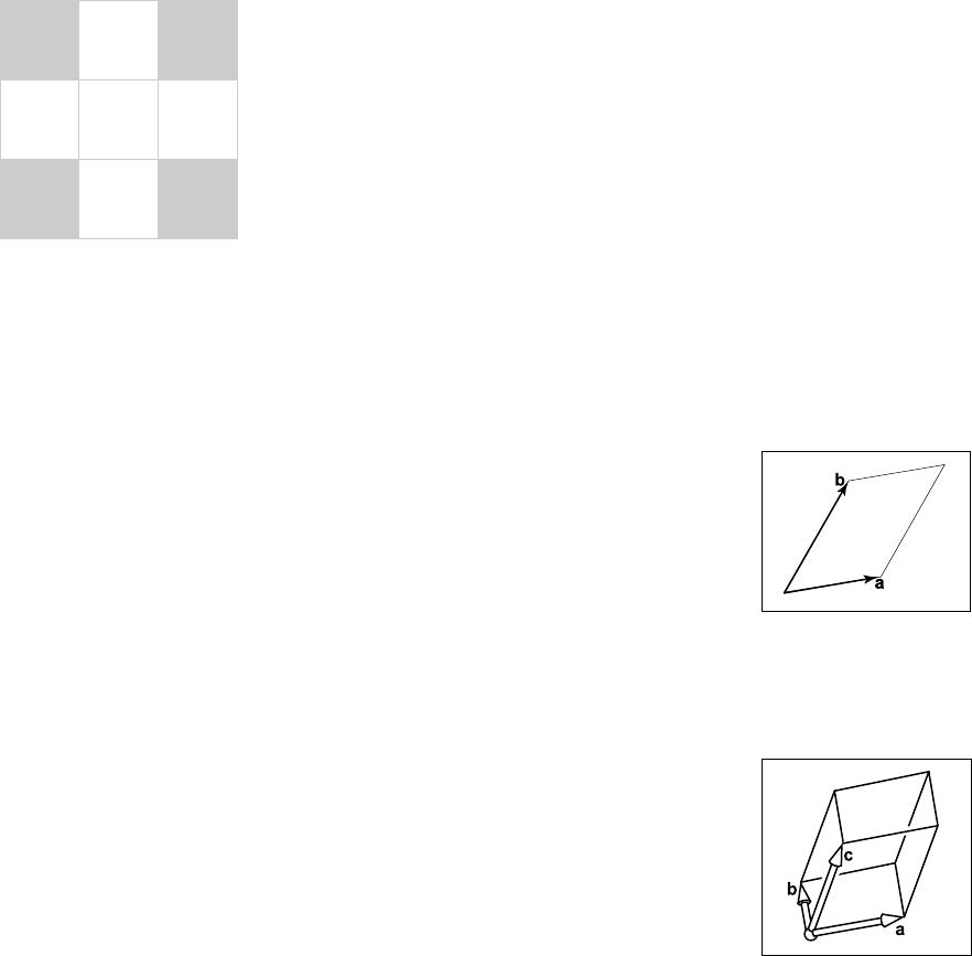
Figure 5.1. The signed
area of the parallelogram is
|ab|, and in this case the
area is positive.
chapter, we review basic linear algebra from a geometric perspective, focusing on
intuition and algorithms that work well in the two- and three-dimensional case.
This chapter can be skipped by readers comfortable with linear algebra. How-
ever, there may be some enlightening tidbits even for such readers, such as the
development of determinants and the discussion of singular and eigenvalue de-
composition.
5.1 Determinants
We usually think of determinants as arising in the solution of linear equations.
However, for our purposes, we will think of determinants as another way to mul-
tiply vectors. For 2D vectors a and b, the determinant |ab| is the area of the
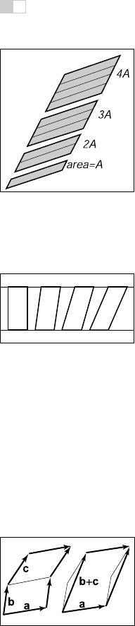
Figure 5.2. The
signed volume of the paral-
lelepiped shown is denoted
by the determinant
|abc|,
and in this case the volume
is positive because the vec-
tors form a right-handed ba-
sis.
parallelogram formed by a and b (Figure 5.1). This is a signed area, and the
sign is positive if a and b are right-handed and negative if they are left-handed.
This means |ab| = −|ba|. In 2D we can interpret “right-handed” as meaning we
rotate the first vector counterclockwise to close the smallest angle to the second
vector. In 3D the determinant must be taken with three vectors at a time. For
three 3D vectors, a, b,andc, the determinant |abc| is the signed volume of the
91
i
i
i
i
i
i
i
i
92 5. Linear Algebra
parallelepiped (3D parallelogram; a sheared 3D box) formed by the three vectors
(Figure 5.2). To compute a 2D determinant, we first need to establish a few of its
properties. We note that scaling one side of a parallelogram scales its area by the
same fraction (Figure 5.3):
|(ka)b| = |a(kb)| = k|ab|.
Also, we note that “shearing” a parallelogram does not change its area (Fig-
ure 5.4):
Figure 5.3. Scaling a par-
allelogram along one direc-
tion changes the area in the
same proportion.
|(a + kb)b| = |a(b + ka)| = |ab|.
Finally, we see that the determinant has the following property:
|a(b + c)| = |ab|+ |ac|, (5.1)
because as shown in Figure 5.5 we can “slide” the edge between the two parallel-
ograms over to form a single parallelogram without changing the area of either of
the two original parallelograms.
Now let’s assume a Cartesian representation for a and b:
Figure 5.4. Shearing
a parallelogram does not
change its area. These
four parallelograms have
the same length base and
thus the same area.
|ab| = |(x
a
x + y
a
y)(x
b
x + y
b
y)|
= x
a
x
b
|xx| + x
a
y
b
|xy| + y
a
x
b
|yx|+ y
a
y
b
|yy|
= x
a
x
b
(0) + x
a
y
b
(+1) + y
a
x
b
(−1) + y
a
y
b
(0)
= x
a
y
b
− y
a
x
b
.
This simplification uses the fact that |vv | =0for any vector v, because the
parallelograms would all be collinear with v and thus without area.
In three dimensions, the determinantof three 3D vectorsa, b,andc is denoted
|abc|. With Cartesian representations for the vectors, there are analogous rules
for parallelepipeds as there are for parallelograms, and we can do an analogous
expansion as we did for 2D:
|abc| = |(x
a
x + y
a
y + z
a
z)(x
b
x + y
b
y + z
b
z)(x
c
x + y
c
y + z
c
z)|
= x
a
y
b
z
c
− x
a
z
b
y
c
− y
a
x
b
z
c
+ y
a
z
b
x
c
+ z
a
x
b
y
c
− z
a
y
b
x
c
.
Figure 5.5. The geometry
behind Equation 5.1. Both
of the parallelograms on the
left can be sheared to cover
the single parallelogram on
the right.
As you can see, the computation of determinants in this fashion gets uglier as the
dimension increases. We will discuss less error-prone ways to compute determi-
nants in Section 5.3.
Example. Determinants arise naturally when computing the expression for one
vector as a linear combination of two others—for example, if we wish to express
a vector c as a combination of vectors a and b:
c = a
c
a + b
c
b.

i
i
i
i
i
i
i
i
5.2. Matrices 93
Figure 5.6. On the left, the vector c can be represented using two basis vectors as
a
c
a +
b
c
b. On the right, we see that the parallelogram formed by a and c is a sheared version of
the parallelogram formed by
b
c
b and a.
We can see from Figure 5.6 that
|(b
c
b)a| = |ca|,
because these parallelograms are just sheared versions of each other. Solving for
b
c
yields
b
c
=
|ca|
|ba|
.
An analogous argument yields
a
c
=
|bc|
|ba|
.
This is the two-dimensional version of Cramer’s rule which we will revisit in
Section 5.3.2.
5.2 Matrices
A matrix is an array of numeric elements that follow certain arithmetic rules. An
example of a matrix with two rows and three columns is
1.7 −1.24.2
3.04.5 −7.2
.

i
i
i
i
i
i
i
i
94 5. Linear Algebra
Matrices are frequently used in computer graphics for a variety of purposes in-
cluding representation of spatial transforms. For our discussion, we assume the
elements of a matrix are all real numbers. This chapter describes both the mechan-
ics of matrix arithmetic and the determinant of “square” matrices, i.e., matrices
with the same number of rows as columns.
5.2.1 Matrix Arithmetic
A matrix times a constant results in a matrix where each element has been multi-
plied by that constant, e.g.,
2
1 −4
32
=
2 −8
64
.
Matrices also add element by element, e.g.,
1 −4
32
+
22
22
=
3 −2
54
.
For matrix multiplication, we “multiply” rows of the first matrix with columns of
the second matrix:
⎡
⎢
⎢
⎢
⎢
⎢
⎢
⎢
⎣
a
11
... a
1m
.
.
.
.
.
.
a
i1
... a
im
.
.
.
.
.
.
a
r1
... a
rm
⎤
⎥
⎥
⎥
⎥
⎥
⎥
⎥
⎦
⎡
⎢
⎢
⎣
b
11
...
.
.
.
b
m1
...
b
1j
.
.
.
b
mj
... b
1c
.
.
.
... b
mc
⎤
⎥
⎥
⎦
=
⎡
⎢
⎢
⎢
⎢
⎢
⎢
⎣
p
11
... p
1j
... p
1c
.
.
.
.
.
.
.
.
.
p
i1
... p
ij
... p
ic
.
.
.
.
.
.
.
.
.
p
r1
... p
rj
... p
rc
⎤
⎥
⎥
⎥
⎥
⎥
⎥
⎦
So the element p
ij
of the resulting product is
p
ij
= a
i1
b
1j
+ a
i2
b
2j
+ ···+ a
im
b
mj
. (5.2)
Taking a product of two matrices is only possible if the number of columns of the
left matrix is the same as the number of rows of the right matrix. For example,
⎡
⎣
01
23
45
⎤
⎦
6789
0123
=
⎡
⎣
0123
12 17 22 27
24 33 42 51
⎤
⎦
.
Matrix multiplication is not commutative in most instances:
AB = BA. (5.3)
i
i
i
i
i
i
i
i
5.2. Matrices 95
Also, if AB = AC, it does not necessarily follow that B = C. Fortunately,
matrix multiplication is associative and distributive:
(AB)C = A(BC),
A(B + C)=AB + AC,
(A + B)C = AC + BC.
5.2.2 Operations on Matrices
We would like a matrix analog of the inverse of a real number. We know the
inverse of a real number x is 1/x and that the product of x and its inverse is 1.
We need a matrix I that we can think of as a “matrix one.” This exists only for
square matrices and is known as the identity matrix; it consists of ones down the
diagonal and zeroes elsewhere. For example, the four by four identity matrix is
I =
⎡
⎢
⎢
⎣
1000
0100
0010
0001
⎤
⎥
⎥
⎦
.
The inverse matrix A
−1
of a matrix A is the matrix that ensures AA
−1
= I.
For example,
12
34
−1
=
−2.01.0
1.5 −0.5
because
12
34
−2.01.0
1.5 −0.5
=
10
01
.
Note that the inverse of A
−1
is A.SoAA
−1
= A
−1
A = I.Theinverseofa
product of two matrices is the product of the inverses, but with the order reversed:
(AB)
−1
= B
−1
A
−1
. (5.4)
We will return to the question of computing inverses later in the chapter.
The transpose A
T
of a matrix A has the same numbers but the rows are
switched with the columns. If we label the entries of A
T
as a
ij
then
a
ij
= a
ji
.
For example,
⎡
⎣
12
34
56
⎤
⎦
T
=
135
246
.
..................Content has been hidden....................
You can't read the all page of ebook, please click here login for view all page.