
i
i
i
i
i
i
i
i
17.5. Physics-Based Animation 433
ing locations are commonly chosen near joints, but, of course, they still lie on skin
surface and not at points where actual bones meet. Therefore, some additional
care and a bit of extra processing is necessary to convert recorded positions into
those of the physical skeleton joints. For example, putting two markers on oppo-
site sides of the elbow or ankle allows the system to obtain better joint position
by averaging locations of the two markers. Without such extra care, very notice-
able artifacts can appear due to offset joint positions as well as inherent noise
and insufficient measurement accuracy. Because of physical inaccuracy during
motion, for example, character limbs can loose contact with objects they are sup-
posed to touch during walking or grasping, problems like foot-sliding (skating)
of the skeleton can occur. Most of these problems can be corrected by using in-
verse kinematics techniques which can explicitly force the required behavior of
the limb’s end.
Recovered joint positions can now be directly applied to the skeleton of a
computer-generated character. This procedure assumes that the physical dimen-
sions of the character are identical to those of the performer. Retargeting recorded
motion to a different character and, more generally, editing MC data, requires
significant care to satisfy necessary constraints (such as maintaining feet on the
ground or not allowing an elbow to bend backwards) and preserve an overall nat-
ural appearance of the modified motion. Generally, the greater the desired change
from the original, the less likely it will be possible to maintain the quality of the
result. An interesting approach to the problem is to record a large collection of
motions and stich together short clips from this library to obtain desired move-
ment. Although this topic is currently a very active research area, limited ability
to adjust the recorded motion to the animator’s needs remains one of the main
disadvantages of motion capture technique.
17.5 Physics-Based Animation
The world around us is governed by physical laws many of which can be formal-
ized as sets of partial or, in some simpler cases, ordinary differential equations.
One of the original applications of computers was (and remains) solving such
equations. It is therefore only natural to attempt to use numerical techniques
developed over the several past decades to obtain realistic motion for computer
animation.
Because of its relative complexity and significant cost, physics-based anima-
tion is most commonly used in situations when other techniques are either un-
available or do not produce sufficiently realistic results. Prime examples include

i
i
i
i
i
i
i
i
434 17. Computer Animation
animation of fluids (which includes many gaseous phase phenomena described
by the same equations—smoke, clouds, fire, etc.), cloth simulation (an exam-
Figure 17.22. Real-
istic cloth simulation is of-
ten performed with physics-
based methods. In this ex-
ample, forces are due to
collisions and gravity.
ple is shown in Figure 17.22), rigid body motion, and accurate deformation of
elastic objects. Governing equations and details of commonly used numerical
approaches are different in each of these cases, but many fundamental ideas and
difficulties remain applicable across applications. Many methods for numerically
solving ODEs and PDEs exist but discussing them in details is far beyond the
scope of this book. To give the reader a flavor of physics-based techniques and
some of the issues involved, we will briefly mention here only the finite differ-
ence approach—one of the conceptually simplest and most popular families of
algorithms which has been applied to most, if not all, differential equations en-
countered in animation.
The key idea of this approach is to replace a differential equation with its dis-
crete analog—a difference equation. To do this, the continuous domain of interest
is represented by a finite set of points at which the solution will be computed. In
the simplest case, these are defined on a uniform rectangular grid as shown in Fig-
ure 17.23. Every derivative present in the original ODE or PDE is then replaced
by its approximation through function values at grid points. One way of doing
this is to subtract the function value at a given point from the function value for
its neighboring point on the grid:
df (t)
dt
≈
Δf
Δt
=
f(t +Δt) − f(t)
Δt
or
∂f(x, t)
∂x
≈
Δf
Δx
=
f(x +Δx, t) − f (x, t)
Δx
.
(17.2)
Figure 17.23. Two possible difference schemes for an equation involving derivatives ∂
f
/∂
x
and ∂
f
/∂
t
. (Left) An explicit scheme expresses unknown values (open circles) only through
known values at the current (black circles) and possibly past (gray circles) time; (Right) Im-
plicit schemes mix known and unknown values in a single equation making it necessary to
solve all such equations as a system. For both schemes, information about values on the
right boundary is needed to close the process.
i
i
i
i
i
i
i
i
17.5. Physics-Based Animation 435
These expressions are, of course, not the only way. One can, for example, use
f(t − Δt) instead of f(t) above and divide by 2Δt. For an equation containing
a time derivative, it is now possible to propagate values of an unknown function
forward in time in a sequence of Δt-size steps by solving the system of difference
equations (one at each spatial location) for unknown f (t +Δt). Some initial
conditions, i.e., values of the unknown function at t =0, are necessary to start the
process. Other information, such as values on the boundary of the domain, might
also be required depending on the specific problem.
The computation of f(t+Δt) can be done easily for so called explicit schemes
when all other values present are taken at the current time and the only unknown
in the corresponding difference equation f (t +Δt) is expressed through these
known values. Implicit schemes mix values at current and future times and might
use, for example,
f(x +Δx, t +Δt) − f (x, t +Δt)
Δx
as an approximation of
∂f
∂x
. In this case one has to solve a system of algebraic
equations at each step.
The choice of difference scheme can dramatically affect all aspects of the
algorithm. The most obvious among them is accuracy. In the limit Δt → 0
or Δx → 0, expressions of the type in Equation (17.2) are exact, but for finite
step size some schemes allow better approximation of the derivative than others.
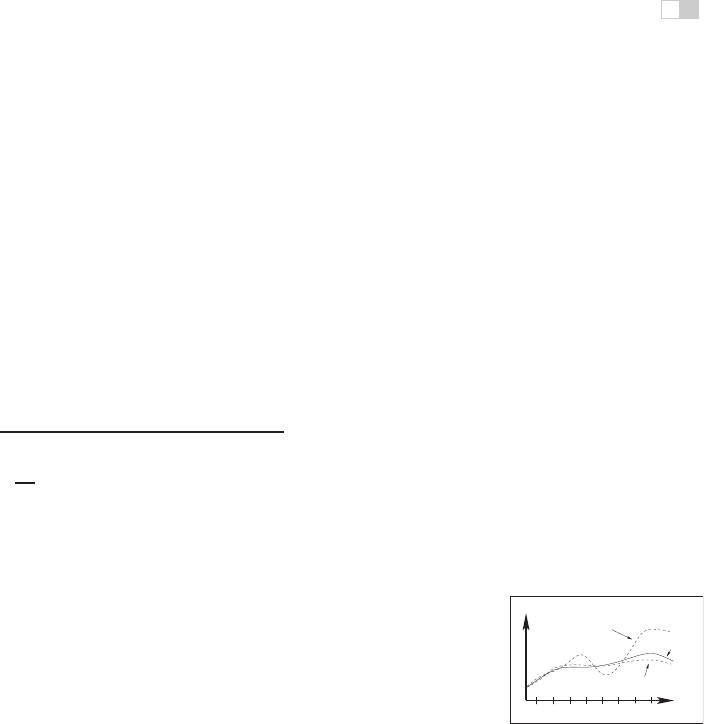
Stability of a difference scheme is related to how fast numerical errors, which are
always present in practice, can grow with time. For stable schemes this growth is
bounded, while for unstable ones it is exponential and can quickly overwhelm the
solution one seeks (see Figure 17.24). It is important to realize that while some
stable
f(t)
t
exact
unstable
Figure 17.24. An unsta-
ble solution might follow the
exact one initially, but can
deviate arbitrarily far from it
with time. Accuracy of a
stable solution might still be
insufficient for a specific ap-
plication.
inaccuracy in the solution is tolerable (and, in fact, accuracy demanded in physics
and engineering is rarely needed for animation), an unstable result is completely
meaningless, and one should avoid using unstable schemes. Generally, explicit
schemes are either unstable or can become unstable at larger step sizes while
implicit ones are unconditionally stable. Implicit schemes allows greater step size
(and, therefore, fewer steps) which is why they are popular despite the need to
solve a system of algebraic equations at each step. Explicit schemes are attractive
because of their simplicity if their stability conditions can be satisfied. Developing
a good difference scheme and corresponding algorithm for a specific problem is
not easy, and for most standard situations it is well advised to use an existing
method. Ample literature discussing details of these techniques is available.
One should remember that, in many cases, just computing all necessary terms
in the equation is a difficult and time-consuming task on its own. In rigid body
or cloth simulation, for example, most of the forces acting on the system are due
i
i
i
i
i
i
i
i
436 17. Computer Animation
to collisions among objects. At each step during animation, one therefore has to
solve a purely geometric, but very non-trivial, problem of collision detection. In
such conditions, schemes which require fewer evaluations of such forces might
provide significant computational savings.
Although the result of solving appropriate time-dependant equations gives
very realistic motion, this approach has its limitations. First of all, it is very
hard to control the result of physics-based animation. Fundamental mathematical
properties of these equations state that once the initial conditions are set, the solu-
tion is uniquely defined. This does not leave much room for animator input and, if
the result is not satisfactory for some reason, one has only a few options. They are
mostly limited to adjusting initial condition used, changing physical properties of
the system, or even modifying the equations themselves by introducing artificial
terms intended to “drive” the solution in the direction the animator wants. Making
such changes requires significant skill as well as understanding of the underlying
physics and, ideally, numerical methods. Without this knowledge, the realism
provided by physics-based animation can be destroyed or severe numerical prob-
lems might appear.
17.6 Procedural Techniques
Imagine that one could write (and implement on a computer) a mathematical func-
tion which outputs precisely the desired motion given some animator guidance.
Physics-based techniques outlined above can be treated as a special case of such
an approach when the “function” involved is the procedure to solve a particular
differential equation and “guidance” is the set of initial and boundary conditions,
extra equation terms, etc.
However, if we are only concerned with the final result, we do not have to
follow a physics-based approach. For example, a simple constant amplitude
wave on the surface of a lake can be directly created by applying the function
f(x,t)=A cos(ωt − kx + φ) with constant frequency ω, wave vector k and
phase φ to get displacement at the 2D point x at time t. A collection of such
waves with random phases and appropriately chosen amplitudes, frequencies, and
wave vectors can result in a very realistic animation of the surface of water with-
out explicitly solving any fluid dynamics equations. It turns out that other rather
simple mathematical functions can also create very interesting patterns or objects.
Several such functions, most based on lattice noises, have been described in Chap-
ter 11. Adding time dependance to these functions allows us to animate certain
complex phenomenamuch easier and cheaper than with physics-based techniques
i
i
i
i
i
i
i
i
17.6. Procedural Techniques 437
while maintaining very high visual quality of the results. If noise(x) is the un-
derlying pattern-generating function, one can create a time-dependant variant of it
by moving the argument position through the lattice. The simplest case is motion
with constant speed: timenoise(x,t)=noise(x + vt), but more complex motion
through the lattice is, of course, also possible and, in fact, more common. One
such path, a spiral, is shown in Figure 17.25. Another approach is to animate pa-
rameters used to generate the noise function. This is especially appropriate if the
appearance changes significantly with time—a cloud becoming more turbulent,
for example. In this way one can animate the dynamic process of formation of
clouds using the function which generates static ones.
t=0
Figure 17.25. A path
through the cube defin-
ing procedural noise is tra-
versed to animate the re-
sulting pattern.
For some procedural techniques, time dependance is a more integral compo-
nent. The simplest cellular automata operate on a 2D rectangular grid where
a binary value is stored at each location (cell). To create a time varying pat-
tern, some user-provided rules for modifying these values are repeatedly applied.
Rules typically involve some set of conditions on the current value and that of
the cell’s neighbors. For example, the rules of the popular 2D Game of Life cel-
lular automaton invented in 1970 by British mathematician John Conway are the
following:
1. A dead cell (i.e., binary value at a given location is 0) with exactly three
live neighbors becomes a live cell (i.e., its value set to 1).
2. A live cell with two or three live neighbors stays alive.
3. In all other cases, a cell dies or remains dead.
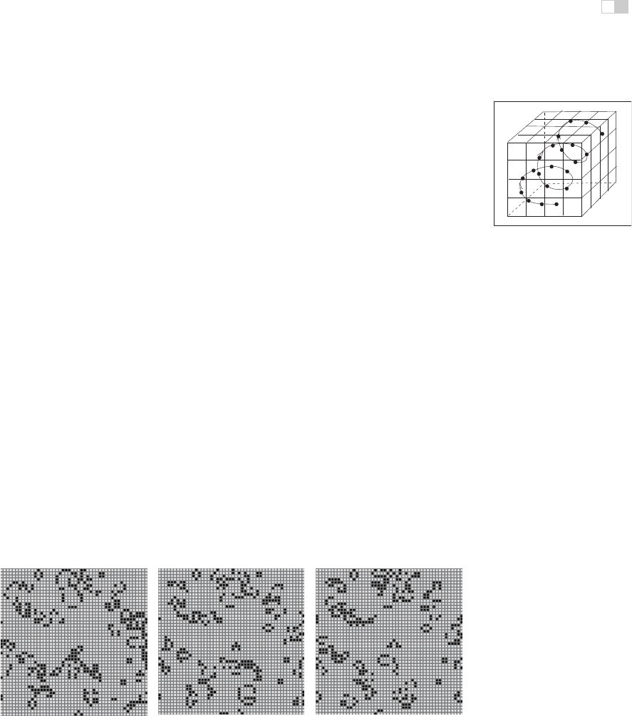
Once the rules are applied to all grid locations, a new pattern is created and a
new evolution cycle can be started. Three sample snapshots of the live cell distri-
bution at different times are shown in Figure 17.26. More sophisticated automata
Figure 17.26. Several (non-consecutive) stages in the evolution of a
Game of Life
automa-
ton. Live cells are shown in black. Stable objects, oscillators, travelling patterns, and many
other interesting constructions can result from the application of very simple rules.
Figure
created using a program by Alan Hensel.
..................Content has been hidden....................
You can't read the all page of ebook, please click here login for view all page.