

i
i
i
i
i
i
i
i
25.5. Rough Layered Model 647
Figure 25.7. Metallic spheres for exponents 10, 100, 1000, 10000 increasing both left-to-
right and top-to-bottom.
chosen to enforce energy conservation and reciprocity. A full rationalization for
the terms is given in the paper by Ashikhmin, listed in the chapter notes.
The specular BRDF of Equation (25.5) is useful for representing metallic sur-
faces where the diffuse component of reflection is very small. Figure 25.7 shows
a set of metal spheres on a texture-mapped Lambertian plane. As the values of
parameters n
u
and n
v
change, the appearance of the spheres shift from rough
metal to almost perfect mirror, and from highly anisotropic to the more familiar
Phong-like behavior.
25.5.2 Diffuse Term for the Anisotropic Phong Model
It is possible to use a Lambertian BRDF together with the anisotropic specular
term; this is done for most models, but it does not necessarily conserve energy. A
i
i
i
i
i
i
i
i
648 25. Reflection Models
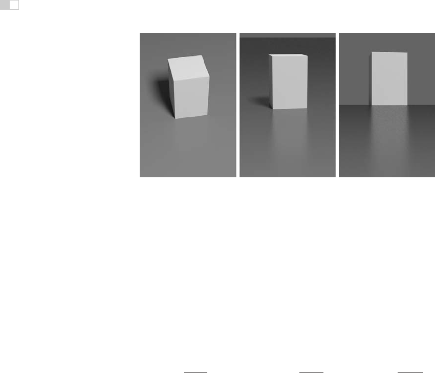
Figure 25.8. Three views for
n
u
=
n
v
= 400 and a diffuse substrate. Note the change in
intensity of the specular reflection.
better approach is a simple angle-dependent form of the diffuse component which
accounts for the fact that the amount of energy available for diffuse scattering
varies due to the dependence of the specular term’s total reflectance on the inci-
dent angle. In particular, diffuse color of a surface disappears near the grazing
angle, because the total specular reflectance is close to one. This well-known ef-
fect cannot be reproduced with a Lambertian diffuse term and is therefore missed
by most reflection models.
Following a similar approach to the coupled model, we can find a form of the
diffuse term that is compatible with the anisotropic Phong lobe:
ρ
d
(k
1
, k
2
)=
28R
d
23π
(1 − R
s
)
&
1 −
1 −
cos θ
i
2
5
'&
1 −
1 −
cos θ
o
2
5
'
.
(25.7)
Here R
d
is the diffuse reflectance for normal incidence, and R
s
is the Phong lobe
coefficient. An example using this model is shown in Figure 25.8.
25.5.3 Implementing the Model
Recall that the BRDF is a combination of diffuse and specular components:
ρ(k
1
, k
2
)=ρ
s
(k
1
, k
2
)+ρ
d
(k
1
, k
2
). (25.8)
The diffuse component is given in Equation (25.7); the specular component is
given in Equation (25.5). It is not necessary to call trigonometric functions to

i
i
i
i
i
i
i
i
25.5. Rough Layered Model 649
compute the exponent, so the specular BRDF can be written:
ρ(k
1
, k
2
)=
(n
u
+1)(n
v
+1)
8π
(n · h)
(n
u
(h·u)
2
+n
v
(h·v)
2
)/(1−(hn)
2
)
(h·k
i
)max(cos θ
i
,cos θ
o
)
F (k
i
·h).
(25.9)
In a Monte Carlo setting, we are interested in the following problem: given k
1
,
generate samples of k
2
with a distribution whose shape is similar to the cosine-
weighted BRDF. Note that greatly undersampling a large value of the integrand is
a serious error, while greatly oversampling a small value is acceptable in practice.
The reader can verify that the densities suggested below have this property.
A suitable way to construct a pdf for sampling is to consider the distribution
of half vectors that would give rise to our BRDF. Such a function is
p
h
(h)=
(n
u
+1)(n
v
+1)
2π
(nh)
n
u
cos
2
φ+n
v
sin
2
φ
, (25.10)
where the constants are chosen to ensure it is a valid pdf.
We can just use the probability density function p
h
(h) of Equation (25.10) to
generate a random h. However, to evaluate the rendering equation, we need both
areflected vector k
o
and a probability density function p(k
o
). It is important to
note that if you generate h according to p
h
(h) and then transform to the resulting
k
o
:
k
o
= −k
i
+2(k
i
·h)h, (25.11)
the density of the resulting k
o
is not p
h
(k
o
). This is because of the difference in
measures in h and k
o
. So the actual density p(k
o
) is
p(k
o
)=
p
h
(h)
4(k
i
h)
. (25.12)
Note that in an implementation where the BRDF is known to be this model, the
estimate of the rendering equation is quite simple as many terms cancel out.
It is possible to generate an h vector whose corresponding vector k
o
will point
inside the surface, i.e., cos θ
o
< 0. The weight of such a sample should be set
to zero. This situation corresponds to the specular lobe going below the horizon
and is the main source of energy loss in the model. Clearly, this problem becomes
progressively less severe as n
u
, n
v
become larger.
The only thing left now is to describe how to generate h vectors with the pdf
of Equation (25.10). We will start by generating h with its spherical angles in
the range (θ, φ) ∈ [0,
π
2
] × [0,
π
2
]. Note that this is only the first quadrant of the
hemisphere. Given two random numbers (ξ
1
,ξ
2
) uniformly distributed in [0, 1],
we can choose
φ =arctan
n
u
+1
n
v
+1
tan
πξ
1
2
, (25.13)
i
i
i
i
i
i
i
i
650 25. Reflection Models
and then use this value of φ to obtain θ according to
cos θ =(1−ξ
2
)
1/(n
u
cos
2
φ+n
v
sin
2
φ+1)
. (25.14)
To sample the entire hemisphere, we use the standard manipulation where ξ
1
is
mapped to one of four possible functions depending on whether it is in [0, 0.25),
[0.25, 0.5), [0.5, 0.75),or[0.75, 1.0). For example for ξ
1
∈ [0.25, 0.5), find φ(1−
4(0.5 −ξ
1
)) via Equation (25.13), and then “flip” it about the φ = π/2 axis. This
ensures full coverage and stratification.
For the diffuse term, use a simpler approach and generate samples according
to a cosine distribution. This is sufficiently close to the complete diffuse BRDF
to substantially reduce variance of the Monte Carlo estimation.
Frequently Asked Questions
• My images look too smooth, even with a complex BRDF. What am I do-
ing wrong?
BRDFs only capture subpixel detail that is too small to be resolved by the eye.
Most real surfaces also have some small variations, such as the wrinkles in skin,
that can be seen. If you want true realism, some sort of texture or displacement
map is needed.
• How do I integrate the BRDF with texture mapping?
Texture mapping can be used to control any parameter on a surface. So any kinds
of colors or control parameters used by a BRDF should be programmable.
• I have very pretty code except for my material class. What am I doing
wrong?
You are probably doing nothing wrong. Material classes tend to be the ugly thing
in everybody’s programs. If you find a nice way to deal with it, please let me
know! My own code uses a shader architecture (Hanrahan & Lawson, 1990)
which makes the material include much of the rendering algorithm.
Notes
There are many BRDF models described in the literature, and only a few of them
have been described here. Others include (Cook & Torrance, 1982; He et al.,
i
i
i
i
i
i
i
i
25.5. Rough Layered Model 651
1992; G. J. Ward, 1992; Oren & Nayar, 1994; Schlick, 1994a; Lafortune et al.,
1997; Stam, 1999; Ashikhmin et al., 2000; Ershov et al., 2001; Matusik et al.,
2003; Lawrence et al., 2004; Stark et al., 2005). The desired characteristics of
BRDF models is discussed in Making Shaders More Physically Plausible (R. R.
Lewis, 1994).
Exercises
1. Suppose that instead of the Lambertian BRDF we used a BRDF of the form
C cos
a
θ
i
. What must C be to conserve energy?
2. The BRDF in Exercise 1 is not reciprocal. Can you modify it to be recipro-
cal?
3. Something like a highway sign is a retroreflector. This means that the
BRDF is large when k
i
and k
o
are near each other. Make a model inspired
by the Phong model that captures retroreflection behavior while being re-
ciprocal and conserving energy.
..................Content has been hidden....................
You can't read the all page of ebook, please click here login for view all page.